Shell Element Responses (Pyvista)¶

[1]:

import openseespy.opensees as ops

import opstool as opst
import opstool.vis.pyvista as opsvis

Model and gravity load¶

[2]:

opst.load_ops_examples("Shell3D")

ops.timeSeries("Linear", 1)
ops.pattern("Plain", 1, 1)
_ = opst.pre.gen_grav_load(direction="Z", factor=-9810)

The original Tcl file comes from http://www.dinochen.com/, and the Python version is converted by opstool.tcl2py().

[3]:

on_notebook = True
jupyter_backend = "static"

# on_notebook = False
# jupyter_backend = None

[4]:

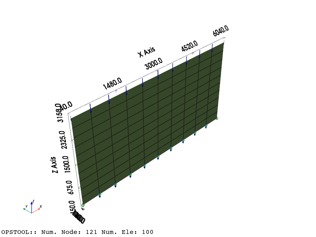
opsvis.set_plot_props(point_size=0, line_width=3, notebook=on_notebook)  # notebook=False for practical use
fig = opsvis.plot_model(show_nodal_loads=True, show_ele_loads=True, show_outline=True)
fig.show(jupyter_backend=jupyter_backend)
# fig.show()

../../../_images/src_vis_pyvista_plot_shell_resp_pyvista_5_0.png

Gravity analysis¶

[5]:

ops.constraints("Transformation")
ops.numberer("RCM")
ops.system("BandGeneral")
ops.test("NormDispIncr", 1.0e-8, 6, 2)
ops.algorithm("Linear")
ops.integrator("LoadControl", 0.1)
ops.analysis("Static")

Save the responses

[6]:

ODB = opst.post.CreateODB(
    odb_tag=1,
    project_gauss_to_nodes="copy",  # project gauss point responses to nodes, optional ["copy", "average", "extrapolate"]
)
for _ in range(10):
    ops.analyze(1)
    ODB.fetch_response_step()
ODB.save_response()

OPSTOOL ::  All responses data with _odb_tag = 1 saved in .opstool.output/RespStepData-1.nc!

Visualize the results¶

Nodal responses, project_gauss_to_nodes needs to be set to “copy”, “average”, or “extrapolate” when creating the ODB

[7]:

opsvis.set_plot_props(cmap="coolwarm_r", show_mesh_edges=True, notebook=on_notebook)

fig = opsvis.plot_unstruct_responses(
    odb_tag=1,
    slides=False,
    step="absMax",
    ele_type="Shell",
    resp_type="sectionForcesAtNodes",  # nodal response, "AtNodes"
    resp_dof="FXX",
)
fig.show(jupyter_backend=jupyter_backend)
# fig.show()

OPSTOOL ::  Loading response data from .opstool.output/RespStepData-1.nc ...

../../../_images/src_vis_pyvista_plot_shell_resp_pyvista_12_1.png

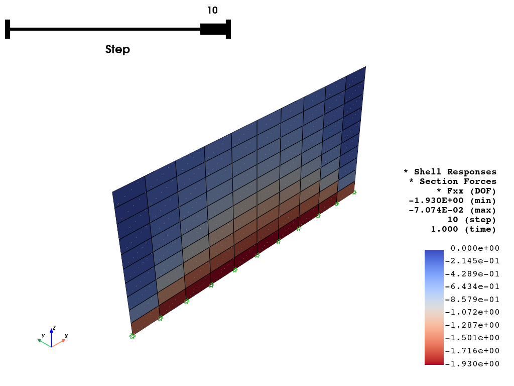
Display the responses at each element, all gauss points will be averaged to the element level.

[8]:

fig = opsvis.plot_unstruct_responses(
    odb_tag=1,
    slides=True,
    ele_type="Shell",
    resp_type="sectionForces",  # element response, "AtGaussPoints", will be averaged to each element
    resp_dof="FXX",
)
fig.show(jupyter_backend=jupyter_backend)

OPSTOOL ::  Loading response data from .opstool.output/RespStepData-1.nc ...

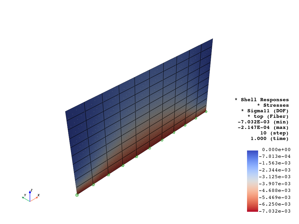
../../../_images/src_vis_pyvista_plot_shell_resp_pyvista_14_1.png

Fiber point stress can be plotted as well, but it requires a shell_fiber_loc to be assigned.

[9]:

fig = opsvis.plot_unstruct_responses(
    odb_tag=1,
    slides=False,
    step="absMax",
    ele_type="Shell",
    resp_type="StressesAtNodes",  # nodal stress response, "AtNodes"
    resp_dof="sigma11",  # sigma11, sigma22, sigma12, sigma13, sigma23
    shell_fiber_loc="top",  # shell_fiber_loc can be "top", "bottom", or "mid" for shell elements, also int
)
fig.show(jupyter_backend=jupyter_backend)

OPSTOOL ::  Loading response data from .opstool.output/RespStepData-1.nc ...

../../../_images/src_vis_pyvista_plot_shell_resp_pyvista_16_1.png

Interacting with Pyvista¶

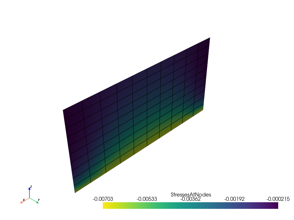
Since version 1.0.18, opstool provides a function get_unstruct_responses_dataset that returns a pyvista UnstructuredGrid so that you can take advantage of all the functionality on it.

[10]:

import pyvista as pv

[11]:

grid = opsvis.get_unstruct_responses_dataset(
    odb_tag=1,
    step="absMax",
    ele_type="Shell",
    resp_type="StressesAtNodes",  # nodal stress response, "AtNodes"
    resp_dof="sigma11",  # sigma11, sigma22, sigma12, sigma13, sigma23
    shell_fiber_loc="top",  # shell_fiber_loc can be "top", "bottom", or "mid" for shell elements, also int
)

OPSTOOL ::  Loading response data from .opstool.output/RespStepData-1.nc ...

[12]:

print(grid)
print("--" * 20)
print(grid.active_scalars_name)

UnstructuredGrid (0x1888f77eaa0)
  N Cells:    100
  N Points:   121
  X Bounds:   0.000e+00, 6.000e+03
  Y Bounds:   0.000e+00, 0.000e+00
  Z Bounds:   0.000e+00, 3.000e+03
  N Arrays:   1
----------------------------------------
StressesAtNodes

[13]:

grid.plot(jupyter_backend=jupyter_backend, show_edges=True, cmap="viridis_r", show_scalar_bar=True)

../../../_images/src_vis_pyvista_plot_shell_resp_pyvista_22_0.png

Plot Over Line¶

[14]:

grid.bounds

[14]:

(0.0, 6000.0, 0.0, 0.0, 0.0, 3000.0)

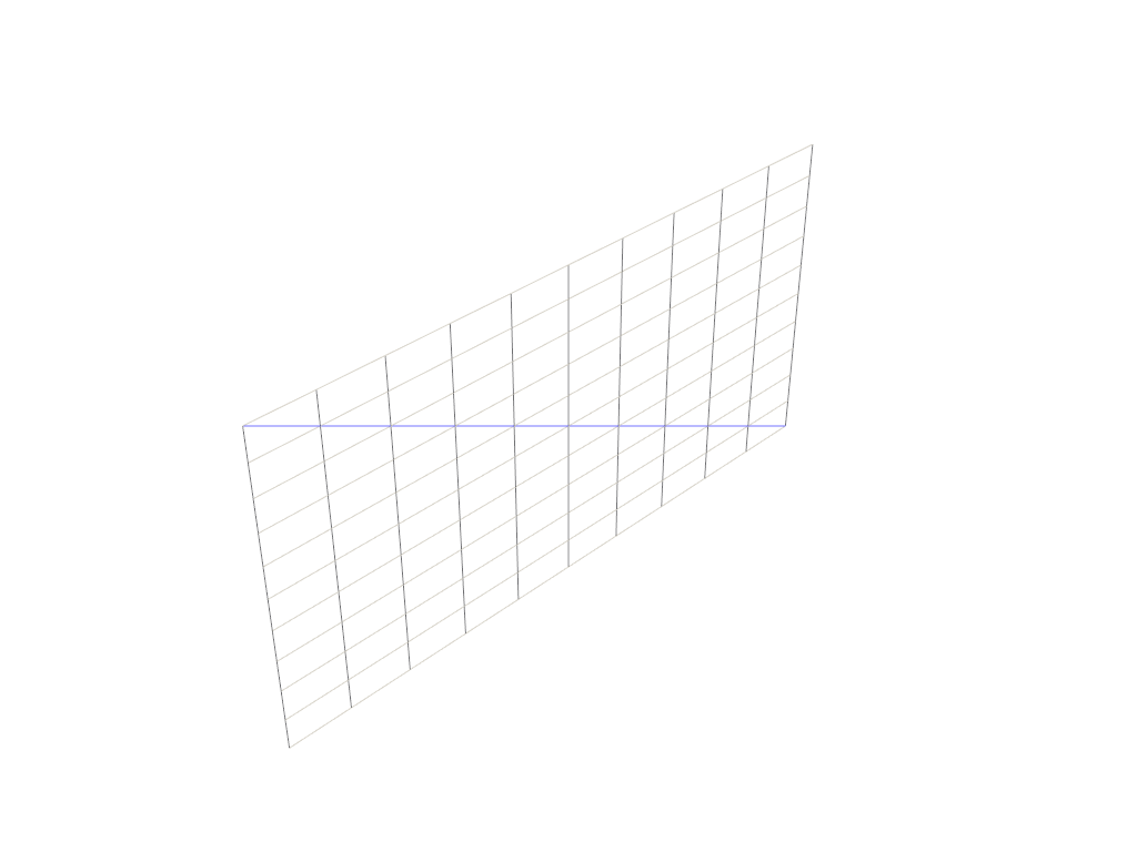
[15]:

a = [0, 0, 0]
b = [6000, 0, 3000]  # A line from (0, 0, 0) to (0, 0, 1)

# Preview how this line intersects this mesh
line = pv.Line(a, b)

p = pv.Plotter()
p.add_mesh(grid, style="wireframe", color="w")
p.add_mesh(line, color="b")
p.show(jupyter_backend=jupyter_backend)

../../../_images/src_vis_pyvista_plot_shell_resp_pyvista_25_0.png

[16]:

grid.plot_over_line(a, b)

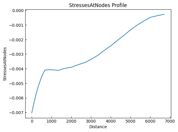
../../../_images/src_vis_pyvista_plot_shell_resp_pyvista_26_0.png

More details can be found in the PyVista Examples.