Gmsh2OPS: Case 1
This case primarily uses the dimension and entity ID information from GMSH to convert the model into an OpenSees format. Refer to the dimensions and entity IDs in Elementary entities vs. physical groups:
[1]:
import opstool as opst
import openseespy.opensees as ops
import gmsh
[2]:
gmsh.initialize()  # Initialize

# Create rectangles with entity tags 1 and 2, the function returns entity IDs
rect1 = gmsh.model.occ.addRectangle(x=0, y=0, z=0, dx=2, dy=3, tag=1)
rect2 = gmsh.model.occ.addRectangle(x=2, y=0, z=0, dx=2, dy=3, tag=2)
# Remove duplicate entities, ensuring overlapping edges between the two rectangles are kept as one
gmsh.model.occ.removeAllDuplicates()
# Synchronize the current Gmsh model, this step is mandatory
gmsh.model.occ.synchronize()

# Get the boundary lines of the two rectangles; dimTags identifies the dimension and entity
lines1 = gmsh.model.getBoundary(dimTags=[(2, rect1)], oriented=False)
lines2 = gmsh.model.getBoundary(dimTags=[(2, rect2)], oriented=False)

# Set mesh division seeds: constrain each boundary line of the rectangles to generate 21 nodes
# Since curves are inherently 1D, only entity IDs are required without specifying dimensions
for l in lines1:
    gmsh.model.mesh.setTransfiniteCurve(tag=l[1], numNodes=21)
for l in lines2:
    gmsh.model.mesh.setTransfiniteCurve(tag=l[1], numNodes=21)
# Constrain mesh generation for the plane as well to ensure internal regularity
# Planes are inherently 2D, so only entity IDs are needed
gmsh.model.mesh.setTransfiniteSurface(tag=rect1)
gmsh.model.mesh.setTransfiniteSurface(tag=rect2)

# Set mesh algorithm, enable RecombineAll (1 for enabling), merging triangular meshes into quadrilateral ones
gmsh.option.setNumber("Mesh.RecombineAll", 1)
gmsh.option.setNumber("Mesh.RecombinationAlgorithm", 1)

# Generate the mesh; since it's for surfaces, dim=2
gmsh.model.mesh.generate(dim=2)

# By default, GMSH generates first-order elements; change the mesh on surface 2 to second-order (nine-node quadrilaterals)
# First, hide surface 1 by setting its visibility to 0
gmsh.option.setNumber("Mesh.MeshOnlyVisible", 1)
gmsh.model.setVisibility(dimTags=[(2, 1)], value=0, recursive=True)
# Then, set the mesh order for all currently visible objects to 2
gmsh.model.mesh.setOrder(2)
# Reactivate surface 1
gmsh.model.setVisibility(dimTags=[(2, 1)], value=1, recursive=True)

# Write the mesh to a file
# gmsh.write("t1.msh")

# Launch the GUI for visualization
# gmsh.fltk.run()
[3]:
ops.wipe()
# Initialize a basic 3D model with 6 degrees of freedom per node
ops.model("basic", "-ndm", 3, "-ndf", 6)

# Define an elastic isotropic material
# Material ID: 1
# Elastic modulus: 2e8
# Poisson's ratio: 0.3
# Density: 7.85
ops.nDMaterial("ElasticIsotropic", 1, 2e8, 0.3, 7.85)

# Define a section using PlateFiber
# Section tag: 1
# Material tag: 1 (linked to the material defined above)
# Thickness: 0.005
secTag = 1
ops.section("PlateFiber", secTag, 1, 0.005)
[4]:
# Initialize GMSH to OpenSeesPy converter with 3D model and 6 degrees of freedom per node
GMSH2OPS = opst.pre.Gmsh2OPS(ndm=3, ndf=6)

# Read the saved .msh file generated by GMSH
# GMSH2OPS.read_gmsh_file("t1.msh")
GMSH2OPS.read_gmsh_data()
# Finalize and close
gmsh.finalize()

# Create OpenSeesPy node commands based on all nodes defined in the GMSH file
GMSH2OPS.create_node_cmds()

# Create OpenSeesPy element commands for specific entities
# ShellMITC4 elements (4-node shell elements)
ele_tags_n4 = GMSH2OPS.create_element_cmds(
    ops_ele_type="ShellMITC4",  # OpenSeesPy element type
    ops_ele_args=[secTag],  # Additional arguments for the element (e.g., section tag)
    dim_entity_tags=[(2, 1)],  # Dimension-entity tags to specify which elements to create
)

# ShellMITC9 elements (9-node shell elements)
ele_tags_n9 = GMSH2OPS.create_element_cmds(
    ops_ele_type="ShellMITC9",  # OpenSeesPy element type for 9-node shells
    ops_ele_args=[secTag],  # Additional arguments for the element (e.g., section tag)
    dim_entity_tags=[(2, 2)],  # Dimension-entity tags to specify which elements to create
)
# Done!
Info:: Geometry Information >>>
15 Entities: 6 Point; 7 Curves; 2 Surfaces; 0 Volumes.

Info:: Physical Groups Information >>>
0 Physical Groups.
Physical Group names: []

Info:: Mesh Information >>>
2101 Nodes; MaxNodeTag 2101; MinNodeTag 1.
946 Elements; MaxEleTag 946; MinEleTag 1.
Using ShellMITC9 - Developed by: Leopoldo Tesser and Diego A. Talledo
[5]:
# Define boundary conditions
# Get the boundary dimension tags for the two surfaces
boundary_dim_tags = GMSH2OPS.get_boundary_dim_tags([(2, 1), (2, 2)])

# Remove the shared boundary between the two surfaces
boundary_dim_tags.remove((1, 2))

# Print the remaining boundary dimension tags
print("Boundary dim_tags:", boundary_dim_tags)

# Create fix commands for the boundary with constraints applied to all 6 degrees of freedom (DOFs)
fix_node_tags = GMSH2OPS.create_fix_cmds(dim_entity_tags=boundary_dim_tags, dofs=[1] * 6)
Boundary dim_tags: [(0, 1), (0, 2), (0, 3), (0, 4), (0, 5), (0, 6), (1, 1), (1, 3), (1, 4), (1, 5), (1, 6), (1, 7)]
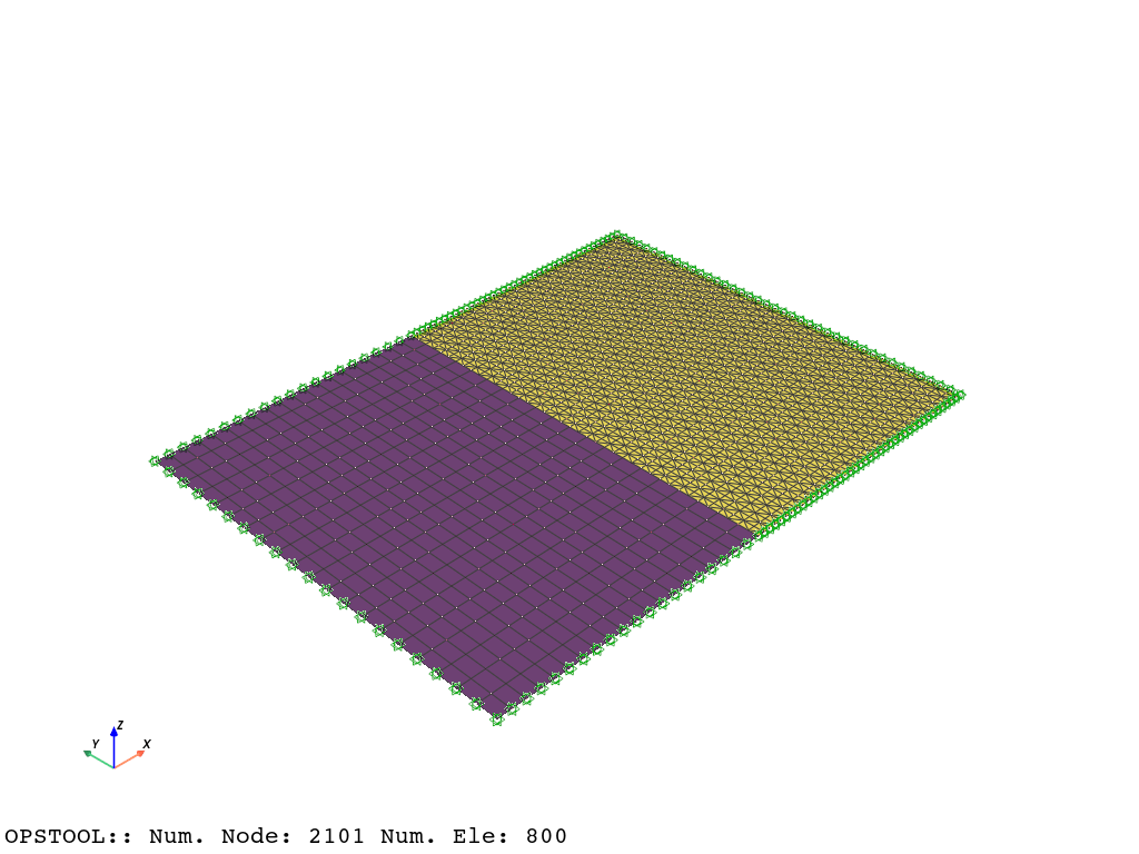
[6]:
opst.vis.pyvista.set_plot_props(point_size=0, notebook=True, mesh_opacity=0.75, cmap_model="viridis")
plotter = opst.vis.pyvista.plot_model()
plotter.show(jupyter_backend="jupyterlab")
# plotter.show()
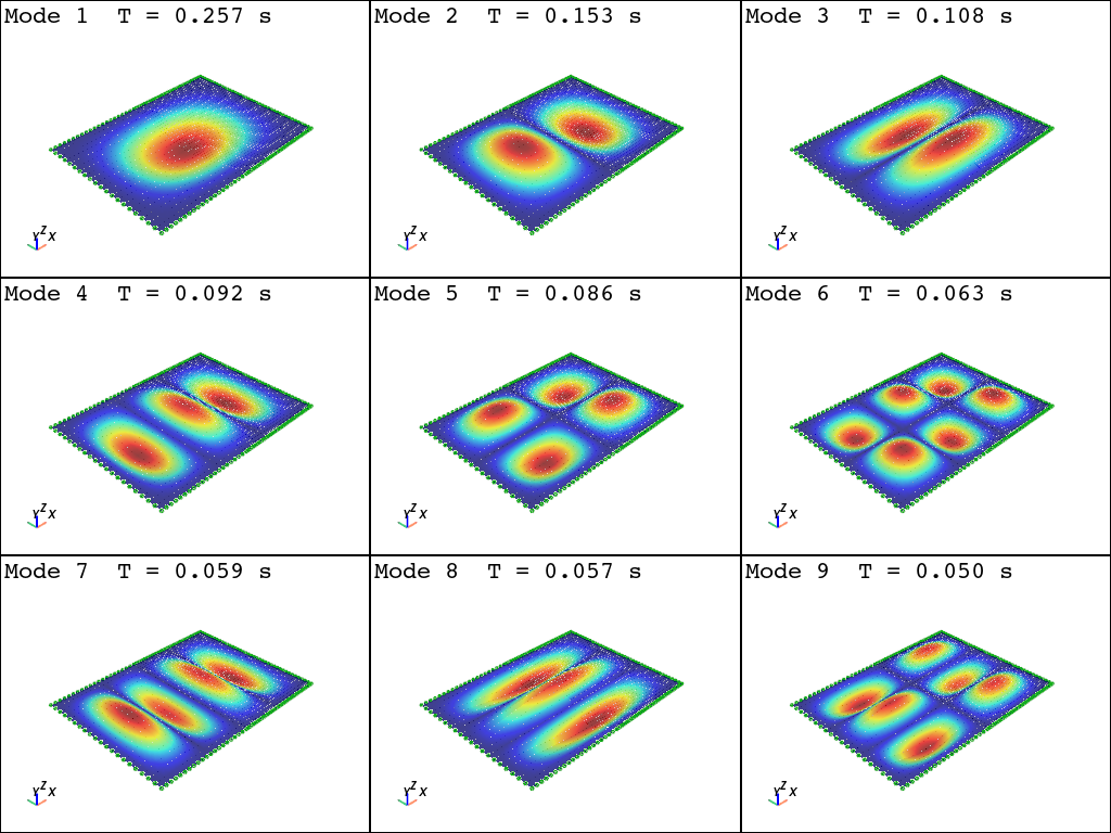
[7]:
opst.vis.pyvista.set_plot_props(show_mesh_edges=False, notebook=True)
plotter = opst.vis.pyvista.plot_eigen([1, 9], subplots=True)

plotter.show(jupyter_backend="jupyterlab")
# plotter.show()
Using DomainModalProperties - Developed by: Massimo Petracca, Guido Camata, ASDEA Software Technology
OPSTOOL :: Eigen data has been saved to .opstool.output/EigenData-Auto.nc!