Unit conversion in post-processing
This feature is available from version 1.0.14.
This document shows how to use opstool to perform unit conversion.
To maintain the flexibility of using OpenSeesPy, opstool implements unit conversion methods in both pre-processing and post-processing.
Pre-processing: opstool.pre.UnitSystem
Post-processing: opstool.post.update_unit_system
Note that these two do not need to be run at the same time.
[1]:
import matplotlib.pyplot as plt
import numpy as np
import openseespy.opensees as ops

import opstool as opst
We use the following two-dimensional truss structure:
model
We use Automatic Unit Conversion to set the basic unit used by the model, which is the lowest level unit system. Then we can easily define the units of various physical quantities.
[2]:
def model(length_unit, force_unit):
    UNIT = opst.pre.UnitSystem(length=length_unit, force=force_unit)
    ops.wipe()
    ops.model("basic", "-ndm", 2, "-ndf", 2)
    # create nodes
    ops.node(1, 0, 0)
    ops.node(2, 144.0 * UNIT.cm, 0)
    ops.node(3, 2.0 * UNIT.m, 0)
    ops.node(4, 80.0 * UNIT.cm, 96.0 * UNIT.cm)
    ops.mass(4, 100 * UNIT.kg, 100 * UNIT.kg)
    # set boundary condition
    ops.fix(1, 1, 1)
    ops.fix(2, 1, 1)
    ops.fix(3, 1, 1)
    # define materials
    ops.uniaxialMaterial("Elastic", 1, 3000.0 * UNIT.N / UNIT.cm2)
    # define elements
    ops.element("Truss", 1, 1, 4, 100.0 * UNIT.cm2, 1)
    ops.element("Truss", 2, 2, 4, 50.0 * UNIT.cm2, 1)
    ops.element("Truss", 3, 3, 4, 50.0 * UNIT.cm2, 1)

    # create TimeSeries
    ops.timeSeries("Linear", 1)
    ops.pattern("Plain", 1, 1)
    ops.load(4, 10.0 * UNIT.kN, -5.0 * UNIT.kN)
We use N and mm as basic units
[3]:
model(length_unit="mm", force_unit="N")
analysis
[4]:
# ------------------------------
# Start of analysis generation
# ------------------------------
ops.system("BandSPD")
ops.numberer("RCM")
ops.constraints("Plain")
ops.integrator("LoadControl", 1.0 / 10)
ops.algorithm("Linear")
ops.analysis("Static")
Response saving
[5]:
odb = opst.post.CreateODB(odb_tag=1)
for _ in range(10):
    ops.analyze(1)
    odb.fetch_response_step()
odb.save_response()
OPSTOOL :: All responses data with _odb_tag = 1 saved in .opstool.output/RespStepData-1.nc!
Post-processing
Original unit system
Since the basic units selected earlier are N and mm units, the response data is naturally presented in this system.
[6]:
node_resp = opst.post.get_nodal_responses(odb_tag=1)
ele_resp = opst.post.get_element_responses(odb_tag=1, ele_type="Truss")
OPSTOOL :: Loading all response data from .opstool.output/RespStepData-1.nc ...
OPSTOOL :: Loading Truss response data from .opstool.output/RespStepData-1.nc ...
[7]:
# fig = opst.vis.pyvista.plot_truss_responses(odb_tag=1, resp_type="axialForce")
# fig.show()
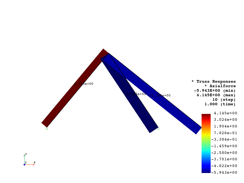
We can visualize the axial force in N
[8]:
opst.vis.pyvista.set_plot_props(notebook=True)
opst.vis.pyvista.set_plot_colors(truss="black")

fig = opst.vis.pyvista.plot_truss_responses(odb_tag=1, resp_type="axialForce")
fig.show(jupyter_backend="")
OPSTOOL :: Loading response data from .opstool.output/RespStepData-1.nc ...

Visualize stress, unit corresponds to MPa (\(N/mm^2\))
[9]:
fig = opst.vis.pyvista.plot_truss_responses(odb_tag=1, resp_type="Stress")
fig.show(jupyter_backend="")
OPSTOOL :: Loading response data from .opstool.output/RespStepData-1.nc ...

Unit conversion in post-processing
We can now update the unit system in the post-processing.
Note that pre must correspond to the base unit system selected earlier (this is a fact).
post is the target unit system to transform to, which can be anything.
All conversions are done automatically inside opstool 😀
[10]:
opst.post.update_unit_system(
    pre={"length": "mm", "force": "N"},
    post={"length": "m", "force": "kN"},
)
After the update, we visualize the axial force, which is kN at this time. We can see that it is 1000 times smaller than before, which is what we expected.
[11]:
fig = opst.vis.pyvista.plot_truss_responses(odb_tag=1, resp_type="axialForce")
fig.show(jupyter_backend="")
OPSTOOL :: Loading response data from .opstool.output/RespStepData-1.nc ...
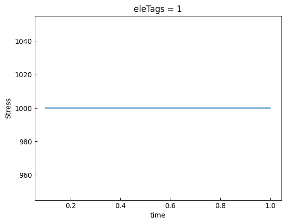
The stress changes from MPa to kPa, which is amplified 1000 times.
[12]:
fig = opst.vis.pyvista.plot_truss_responses(odb_tag=1, resp_type="Stress")
fig.show(jupyter_backend="")
OPSTOOL :: Loading response data from .opstool.output/RespStepData-1.nc ...

Plot ratio coefficient
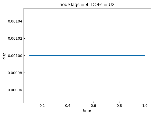
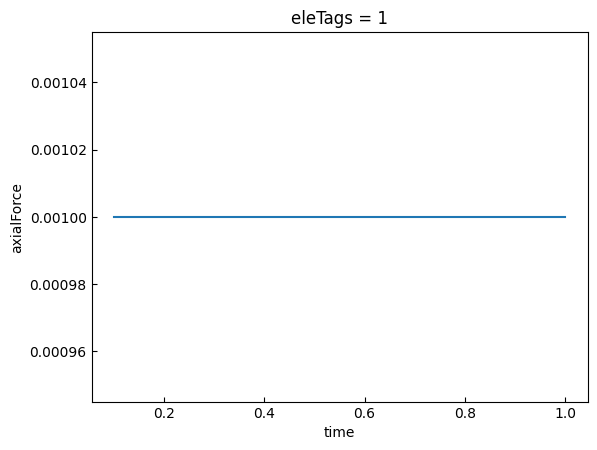
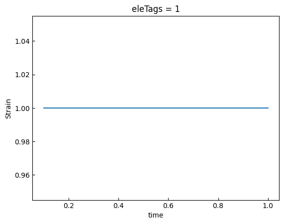
Let’s look at the unit conversion factors for displacement, axial force, stress, and strain. Note that strain is dimensionless.
[13]:
node_resp2 = opst.post.get_nodal_responses(odb_tag=1)
ele_resp2 = opst.post.get_element_responses(odb_tag=1, ele_type="Truss")
OPSTOOL :: Loading all response data from .opstool.output/RespStepData-1.nc ...
OPSTOOL :: Loading Truss response data from .opstool.output/RespStepData-1.nc ...
[14]:
disp = node_resp["disp"].sel(nodeTags=4, DOFs="UX")
disp2 = node_resp2["disp"].sel(nodeTags=4, DOFs="UX")

(disp2 / disp).plot.line(x="time")
plt.show()
[15]:
force = ele_resp["axialForce"].sel(eleTags=1)
force2 = ele_resp2["axialForce"].sel(eleTags=1)

(force2 / force).plot.line(x="time")
plt.show()
[16]:
stress = ele_resp["Stress"].sel(eleTags=1)
stress2 = ele_resp2["Stress"].sel(eleTags=1)
ratio = np.round(stress2 / stress, 3)

(ratio).plot.line(x="time")
plt.show()
[17]:
strain = ele_resp["Strain"].sel(eleTags=1)
strain2 = ele_resp2["Strain"].sel(eleTags=1)
ratio = np.round(strain2 / strain, 3)

(ratio).plot.line(x="time")
plt.show()
Reset unit system
If you wish to reset to the original unit system, you can:
[18]:
opst.post.reset_unit_system()