Node Response¶

[1]:

import matplotlib.pyplot as plt
import numpy as np
import openseespy.opensees as ops

import opstool as opst

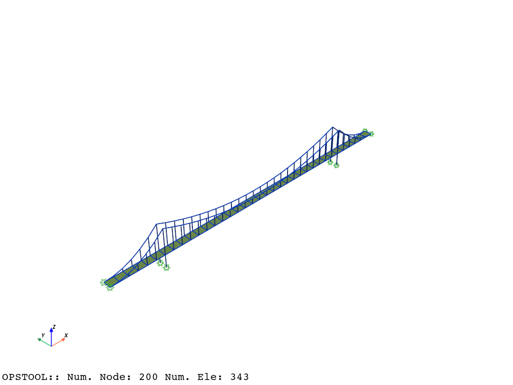
We load a suspension bridge model and visualize it:

[2]:

opst.load_ops_examples("suspensionbridge")  # or your model code here

# plot
opst.vis.pyvista.set_plot_props(notebook=True)  # set notebook=False for practical use
fig = opst.vis.pyvista.plot_model(show_nodal_loads=True, show_ele_loads=True)
fig.show(jupyter_backend="static")  # fig.show() for practical use

../../_images/src_post_nodal_resp_3_0.png

Result Saving¶

Next, we define gravity loads and perform the analysis The opstool.pre.gen_grav_load() function assists in generating gravity loads based on the current node masses. Of course, you can define the loads in your own way.

[3]:

ops.timeSeries("Linear", 1)
ops.pattern("Plain", 1, 1)
_ = opst.pre.gen_grav_load(direction="Z", factor=-9.81)

[4]:

ops.system("BandGeneral")
# Create the constraint handler, the transformation method
ops.constraints("Transformation")
# Create the DOF numberer, the reverse Cuthill-McKee algorithm
ops.numberer("RCM")
# Create the convergence test, the norm of the residual with a tolerance of
# 1e-12 and a max number of iterations of 10
ops.test("NormDispIncr", 1.0e-12, 10, 3)
# Create the solution algorithm, a Newton-Raphson algorithm
ops.algorithm("Newton")
# Create the integration scheme, the LoadControl scheme using steps of 0.1
ops.integrator("LoadControl", 0.1)
# Create the analysis object
ops.analysis("Static")

opstool allows us to save the data at each step of the analysis! First, we create a database class using opstool.post.CreateODB, and then, during each step of the analysis, we call its method .fetch_response_step to retrieve the data for the current step. Once all the analysis steps are completed, we use the .save_response method to save the data in one go.

Note

The data-saving method here is generic. It enables saving all types of result data, including nodes, elements, and more, in one go. Additionally, it is analysis-independent, functioning consistently for both static and dynamic analyses.

[5]:

ODB = opst.post.CreateODB(odb_tag=1)
for _ in range(10):
    ops.analyze(1)
    ODB.fetch_response_step()
ODB.save_response()

OPSTOOL ::  All responses data with _odb_tag = 1 saved in .opstool.output/RespStepData-1.nc!

Result Reading¶

The provided function opstool.post.get_nodal_responses() make it easy to read node responses. Supported response types include:

“disp” - Displacement at the node.
“vel” - Velocity at the node.
“accel” - Acceleration at the node.
“reaction” - Reaction forces at the node.
“reactionIncInertia” - Reaction forces including inertial effects.
“rayleighForces” - Forces resulting from Rayleigh damping.
“pressure” - Pressure applied to the node.

Data is saved as an xarray.DataArray structure, which facilitates more user-friendly data handling.

Displacement¶

For example, to read displacements, you can use the following:

[6]:

node_disp = opst.post.get_nodal_responses(odb_tag=1, resp_type="disp")

OPSTOOL ::  Loading disp response data from .opstool.output/RespStepData-1.nc ...

[7]:

node_disp.dims

[7]:

('time', 'nodeTags', 'DOFs')

To retrieve the coordinates for each dimension, you can use the following:

[8]:

print(node_disp.coords["time"].data)
print()
print(node_disp.coords["DOFs"].data)
print()
print(node_disp.coords["nodeTags"].data)

[0.  0.1 0.2 0.3 0.4 0.5 0.6 0.7 0.8 0.9 1. ]

['UX' 'UY' 'UZ' 'RX' 'RY' 'RZ']

[  1   2   3   4   5   6   7   8   9  10  11  12  13  14  15  16  17  18
  19  20  21  22  23  24  25  26  27  28  29  30  31  32  33  34  35  36
  37  38  39  40  41  42  43  44  45  46  47  48  49  50  51  52  53  54
  55  56  57  58  59  60  61  62  63  64  65  66  67  68  69  70  71  72
  73  74  75  76  77  78  79  80  81  82  83  84  85  86  87  88  89  90
  91  92  93  94  95  96  97  98  99 100 101 102 103 104 105 106 107 108
 109 110 111 112 113 114 115 116 117 118 119 120 121 122 123 124 125 126
 127 128 129 130 131 132 133 134 135 136 137 138 139 140 141 142 143 144
 145 146 147 148 149 150 151 152 153 154 155 156 157 158 159 160 161 162
 163 164 165 166 167 168 169 170 171 172 173 174 175 176 177 178 179 180
 181 182 183 184 185 186 187 188 189 190 191 192 193 194 195 196 197 198
 199 200]

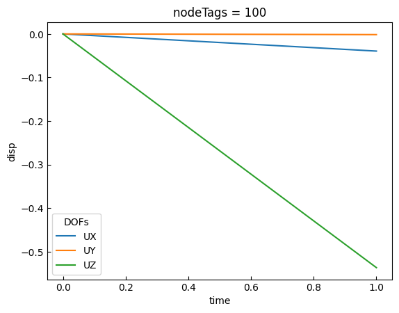
The .sel method can be used to retrieve specific elements corresponding to a particular dimension. For example, the following code retrieves the three translational displacements of node 100:

[9]:

data = node_disp.sel(nodeTags=100, DOFs=["UX", "UY", "UZ"])
data.plot.line(x="time")
plt.show()

../../_images/src_post_nodal_resp_20_0.png

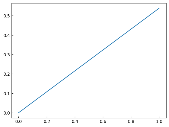
We can also perform array operations using libraries like NumPy. For example, the following code computes the L2 norm:

[10]:

times = node_disp.coords["time"].data
disp = np.linalg.norm(data, axis=-1)
plt.plot(times, disp)
plt.show()

../../_images/src_post_nodal_resp_22_0.png

Reaction forces¶

We can also retrieve reaction forces and perform operations on them. For example:

[11]:

node_react = opst.post.get_nodal_responses(odb_tag=1, resp_type="reaction")

OPSTOOL ::  Loading reaction response data from .opstool.output/RespStepData-1.nc ...

[12]:

node_react

In practice, we are more interested in computing the total reaction force. This can be achieved by applying a summation method. The provided nodeTags dimension indicates that the summation is performed over all nodes.

For example:

[13]:

node_react = node_react.sum(dim="nodeTags", skipna=True)
node_react

Since gravity loads are applied in the Z direction, we retrieve the total reaction forces in the Z direction:

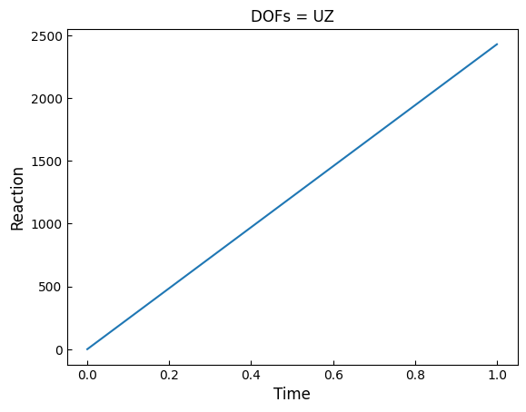
[14]:

node_react_uz = node_react.sel(DOFs="UZ")
node_react_uz.plot.line(x="time")
plt.xlabel("Time", fontsize=12)
plt.ylabel("Reaction", fontsize=12)
plt.show()

../../_images/src_post_nodal_resp_30_0.png