Smart Analysis
API :: opstool.anlys.SmartAnalyze
[1]:
import openseespy.opensees as ops

import opstool as opst
Reinforced Concrete Frame Pushover Analysis
Moddling
[2]:
def model():
    ops.wipe()
    ops.model("basic", "-ndm", 3, "-ndf", 6)
    width = 360.0
    height = 144.0
    ops.node(1, 0.0, 0.0, 0.0)
    ops.node(2, width, 0.0, 0.0)
    ops.node(3, 0.0, 0.0, height)
    ops.node(4, width, 0.0, height)
    ops.fix(1, 1, 1, 1, 1, 1, 1)
    ops.fix(2, 1, 1, 1, 1, 1, 1)

    ops.uniaxialMaterial("Concrete01", 1, -6.0, -0.004, -5.0, -0.014)
    ops.uniaxialMaterial("Concrete01", 2, -5.0, -0.002, 0.0, -0.006)

    fy = 60.0
    E = 30000.0
    ops.uniaxialMaterial("Steel01", 3, fy, E, 0.01)

    # Define cross-section for nonlinear columns
    # ------------------------------------------
    colWidth = 15
    colDepth = 24
    cover = 1.5
    As = 0.60  # area of no. 7 bars
    # some variables derived from the parameters
    y1 = colDepth / 2.0
    z1 = colWidth / 2.0

    ops.section("Fiber", 1, "-GJ", 1000000)
    ops.patch("rect", 1, 10, 10, cover - y1, cover - z1, y1 - cover, z1 - cover)
    # Create the concrete cover fibers (top, bottom, left, right)
    ops.patch("rect", 2, 11, 1, -y1, z1 - cover, y1, z1)
    ops.patch("rect", 2, 11, 1, -y1, -z1, y1, cover - z1)
    ops.patch("rect", 2, 1, 10, -y1, cover - z1, cover - y1, z1 - cover)
    ops.patch("rect", 2, 1, 10, y1 - cover, cover - z1, y1, z1 - cover)
    # Create the reinforcing fibers (left, middle, right)
    ops.layer("straight", 3, 5, As, y1 - cover, z1 - cover, y1 - cover, cover - z1)
    ops.layer("straight", 3, 2, As, 0.0, z1 - cover, 0.0, cover - z1)
    ops.layer("straight", 3, 5, As, cover - y1, z1 - cover, cover - y1, cover - z1)

    # Define column elements
    # ----------------------
    ops.geomTransf("PDelta", 1, -1, 0, 0)
    # Number of integration points along length of element
    np = 5
    # Lobatto integratoin
    ops.beamIntegration("Lobatto", 1, 1, np)
    eleType = "forceBeamColumn"
    ops.element(eleType, 1, 1, 3, 1, 1)
    ops.element(eleType, 2, 2, 4, 1, 1)

    # Define beam elment
    # -----------------------------
    ops.geomTransf("Linear", 2, 0.0, 0.0, 1.0)
    ops.element("elasticBeamColumn", 3, 3, 4, 360.0, 4030.0, 2015.0, 10000, 8640.0, 8640.0, 2)
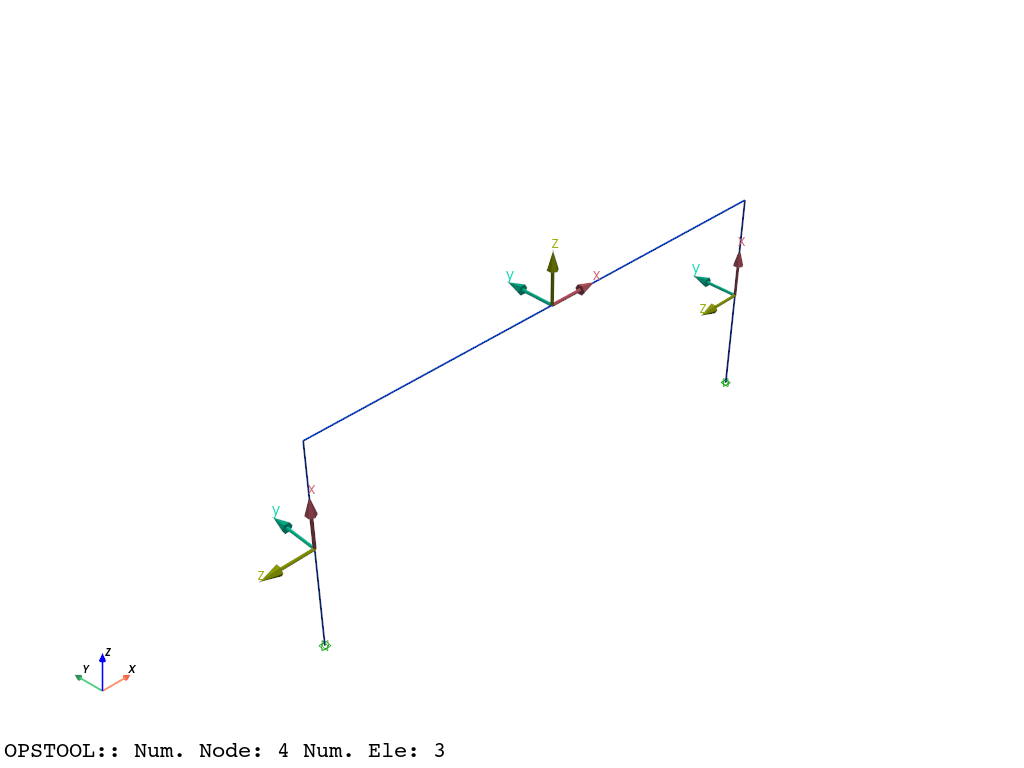
[3]:
model()
opst.vis.pyvista.set_plot_props(notebook=True)  # you should not use
fig = opst.vis.pyvista.plot_model(show_local_axes=True)
fig.show(jupyter_backend="jupyterlab")
# fig.show()
Gravity analysis
[4]:
def gravity_analysis():
    #  a parameter for the axial load
    P = 180.0  # 10% of axial capacity of columns

    # Create a Plain load pattern with a Linear TimeSeries
    ops.timeSeries("Linear", 1)
    ops.pattern("Plain", 1, 1)

    # Create nodal loads at nodes 3 & 4
    #    nd  FX,  FY, MZ
    ops.load(3, 0.0, 0.0, -P, 0.0, 0.0, 0.0)
    ops.load(4, 0.0, 0.0, -P, 0.0, 0.0, 0.0)

    # Start of analysis generation
    # ------------------------------
    ops.system("BandGeneral")
    ops.constraints("Transformation")
    ops.numberer("RCM")
    ops.test("NormDispIncr", 1.0e-12, 10, 3)
    ops.algorithm("Newton")
    ops.integrator("LoadControl", 0.1)
    ops.analysis("Static")
    ops.analyze(10)
Pushover analysis
[5]:
def pushover_load():
    ops.loadConst("-time", 0.0)
    # Define lateral loads
    # --------------------
    # Set some parameters
    H = 10.0  # Reference lateral load
    # Set lateral load pattern with a Linear TimeSeries
    ops.pattern("Plain", 2, 1)
    ops.load(3, H, 0.0, 0.0, 0.0, 0.0, 0.0)
    ops.load(4, H, 0.0, 0.0, 0.0, 0.0, 0.0)
Smart Analysis
No fixed number of analyses
[6]:
# Set some parameters
dU = 0.1  # Displacement increment
maxU = 45.0  # Max displacement
ok = 0
currentDisp = 0

model()
gravity_analysis()
pushover_load()
If tryAddTestTimes is turned on, it will first try to increase the number of test;
if tryAlterAlgoTypes is turned on, it will continue to try to change the iterative algorithm specified by the user;
Then, if it does not converge, it will try to automatically split the step size until the specified minimum step size minStep is reached.
If it still does not converge, the analysis is considered to have failed.
We can see that opensees throws out non-convergence information, but converges successfully when the number of iterations increases to 50.
[7]:
ODB = opst.post.CreateODB(odb_tag=1)  # Create an ODB object to store results

analysis = opst.anlys.SmartAnalyze(
    "Static",
    tryAddTestTimes=True,  # add test times to the analysis
    testIterTimesMore=[50, 100],
    tryAlterAlgoTypes=True,  # try different algorithms
    algoTypes=[40, 10, 20, 30],  # algorithm types to try
    minStep=1e-6,  # minimum step size for substepping
    debugMode=True,  # False for progress bar, True for debug info
    printPer=100,  # print every 100 steps
)

while ok == 0 and currentDisp < maxU:
    #  Perform the analysis one step at a time
    analysis.StaticAnalyze(node=3, dof=1, seg=dU)

    ODB.fetch_response_step()  # Fetch the response for the current step

    currentDisp = ops.nodeDisp(3, 1)

analysis.close()  # Close the analysis object, when analysis steps are unknown

ODB.save_response()

print("🎉 Analysis Completed Successfully 🎉")
>>> ✳️ OPSTOOL::SmartAnalyze:: Setting algorithm to KrylovNewton ...
>>> ✅ OPSTOOL::SmartAnalyze:: progress 100 steps. Time consumption: 0.128 s.
>>> ✅ OPSTOOL::SmartAnalyze:: progress 200 steps. Time consumption: 0.222 s.
>>> ✳️ OPSTOOL::SmartAnalyze:: Adding test times to 50.
>>> ✅ OPSTOOL::SmartAnalyze:: progress 300 steps. Time consumption: 0.348 s.
WARNING: CTestEnergyIncr::test() - failed to converge
after: 10 iterations
 current EnergyIncr: 1.84355e-05 (max: 1e-10)   Norm deltaX: 0.000384464, Norm deltaR: 0.194756
AcceleratedNewton::solveCurrentStep() -The ConvergenceTest object failed in test()
StaticAnalysis::analyze() - the Algorithm failed at step: 0 with domain at load factor 2.89482
OpenSees > analyze failed, returned: -3 error flag
WARNING: CTestEnergyIncr::test() - failed to converge
after: 10 iterations
 current EnergyIncr: 2.70125e-05 (max: 1e-10)   Norm deltaX: 0.000819596, Norm deltaR: 0.253889
AcceleratedNewton::solveCurrentStep() -The ConvergenceTest object failed in test()
StaticAnalysis::analyze() - the Algorithm failed at step: 0 with domain at load factor 1.64367
OpenSees > analyze failed, returned: -3 error flag
>>> ✅ OPSTOOL::SmartAnalyze:: progress 400 steps. Time consumption: 0.442 s.
>>> ✳️ OPSTOOL::SmartAnalyze:: Adding test times to 50.
OPSTOOL :: All responses data with _odb_tag = 1 saved in .opstool.output/RespStepData-1.nc!
🎉 Analysis Completed Successfully 🎉
Analysis of the fixed number of steps
[8]:
# Set some parameters
dU = 0.1  # Displacement increment
maxU = 45.0  # Max displacement

model()
gravity_analysis()
pushover_load()
[9]:
ODB = opst.post.CreateODB(odb_tag=2)  # Create ODB object

analysis = opst.anlys.SmartAnalyze(
    "Static",
    tryAddTestTimes=True,  # add test times to the analysis
    testIterTimesMore=[50, 100],
    tryAlterAlgoTypes=True,  # try different algorithms
    algoTypes=[40, 10, 20, 30],  # algorithm types to try
    minStep=1e-6,  # minimum step size for substepping
    relaxation=0.5,
    debugMode=False,  # False for progress bar, True for debug info
)
segs = analysis.static_split([maxU], dU)  # Tell the analysis how to split the steps, and how many steps to take

for seg in segs:
    analysis.StaticAnalyze(node=3, dof=1, seg=seg)
    ODB.fetch_response_step()  # fetch response for the current step
ODB.save_response()  # save response to ODB
analysis.close()  # Close the analysis object
OPSTOOL::SmartAnalyze: 100%|██████████| 450/450 [00:00<00:00, 625.35 step/s]
Note: OpenSees LogFile has been generated in .SmartAnalyze-OpenSees.log.
>>> 🎉 OPSTOOL::SmartAnalyze:: Successfully finished! Time consumption: 0.733 s. 🎉
OPSTOOL :: All responses data with _odb_tag = 2 saved in .opstool.output/RespStepData-2.nc!
Note
In fact, a suggested solution maybe:
testIterTimes=100,
tryAddTestTimes=True,  # add test times to the analysis
testIterTimesMore=[250, 500, 1000],
tryAlterAlgoTypes=False,  # fix algorithm
algoTypes=[40],  # algorithm is KrylovNewton
relaxation=0.5,
minStep=1e-6,  # minimum step size for substepping
Increasing the number of iterations is often beneficial for KrylovNewton, and has better convergence characteristics. If it does not work, try automatic splitting step size.
Post-processing
Nodal Responses
[10]:
node_resp = opst.post.get_nodal_responses(odb_tag=1)
print(node_resp)
OPSTOOL :: Loading all response data from .opstool.output/RespStepData-1.nc ...
<xarray.Dataset> Size: 269kB
Dimensions:             (time: 451, nodeTags: 4, DOFs: 6)
Coordinates:
  * time                (time) float32 2kB 0.0 0.6715 1.179 ... 1.536 1.519
  * nodeTags            (nodeTags) int32 16B 1 2 3 4
  * DOFs                (DOFs) <U2 48B 'UX' 'UY' 'UZ' 'RX' 'RY' 'RZ'
Data variables:
    disp                (time, nodeTags, DOFs) float32 43kB 0.0 ... 6.499e-15
    vel                 (time, nodeTags, DOFs) float32 43kB 0.0 0.0 ... 0.0 0.0
    accel               (time, nodeTags, DOFs) float32 43kB 0.0 0.0 ... 0.0 0.0
    reaction            (time, nodeTags, DOFs) float32 43kB 1.08e-15 ... -4.9...
    reactionIncInertia  (time, nodeTags, DOFs) float32 43kB 1.08e-15 ... -4.9...
    rayleighForces      (time, nodeTags, DOFs) float32 43kB 0.0 0.0 ... 0.0 0.0
    pressure            (time, nodeTags) float32 7kB 0.0 0.0 0.0 ... 0.0 0.0 0.0
Attributes:
    UX:       Displacement in X direction
    UY:       Displacement in Y direction
    UZ:       Displacement in Z direction
    RX:       Rotation about X axis
    RY:       Rotation about Y axis
    RZ:       Rotation about Z axis
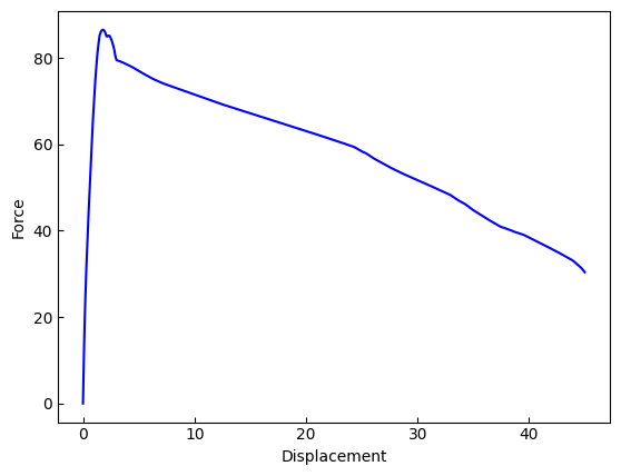
[11]:
node3disp = node_resp["disp"].sel(nodeTags=3, DOFs="UX")
reaction = node_resp["reaction"].sel(DOFs="UX").sum(dim="nodeTags")
[12]:
import matplotlib.pyplot as plt

plt.plot(node3disp, -reaction, c="b")
plt.xlabel("Displacement")
plt.ylabel("Force")
plt.show()
Frame Element Responses
[13]:
frame_resp = opst.post.get_element_responses(odb_tag=1, ele_type="Frame")
frame_resp
OPSTOOL :: Loading Frame response data from .opstool.output/RespStepData-1.nc ...
[13]:
<xarray.Dataset> Size: 771kB
Dimensions:              (time: 451, eleTags: 3, localDofs: 12, basicDofs: 6,
                          secPoints: 7, secDofs: 6, locs: 4)
Coordinates:
  * time                 (time) float32 2kB 0.0 0.6715 1.179 ... 1.536 1.519
  * eleTags              (eleTags) int32 12B 1 2 3
  * localDofs            (localDofs) <U3 144B 'FX1' 'FY1' 'FZ1' ... 'MY2' 'MZ2'
  * basicDofs            (basicDofs) <U3 72B 'N' 'MZ1' 'MZ2' 'MY1' 'MY2' 'T'
  * secPoints            (secPoints) int32 28B 1 2 3 4 5 6 7
  * secDofs              (secDofs) <U2 48B 'N' 'MZ' 'VY' 'MY' 'VZ' 'T'
  * locs                 (locs) <U5 80B 'alpha' 'X' 'Y' 'Z'
Data variables:
    localForces          (time, eleTags, localDofs) float32 65kB -180.0 ... -...
    basicForces          (time, eleTags, basicDofs) float32 32kB -180.0 ... 4...
    basicDeformations    (time, eleTags, basicDofs) float32 32kB -0.01746 ......
    plasticDeformation   (time, eleTags, basicDofs) float32 32kB -0.0003215 ....
    sectionForces        (time, eleTags, secPoints, secDofs) float32 227kB -1...
    sectionDeformations  (time, eleTags, secPoints, secDofs) float32 227kB -0...
    sectionLocs          (time, eleTags, secPoints, locs) float32 152kB 0.0 ....
Attributes:
    localDofs:  local coord system dofs at end 1 and end 2
    basicDofs:  basic coord system dofs at end 1 and end 2
    secPoints:  section points No.
    secDofs:    section forces and deformations Dofs. Note that the section D...
Notes: Note that the deformations are displacements and rotations in...[14]:
frame1defo = frame_resp["sectionDeformations"].sel(eleTags=1, secDofs="MY")
frame1fo = frame_resp["sectionForces"].sel(eleTags=1, secDofs="MY")
frame1defo = frame1defo.dropna(dim="secPoints", how="all")
frame1fo = frame1fo.dropna(dim="secPoints", how="all")
frame1defo.head()
[14]:
<xarray.DataArray 'sectionDeformations' (time: 5, secPoints: 5)> Size: 100B
array([[-2.5559136e-21, -1.4624082e-21, -1.5771168e-22,  2.1066618e-22,
         6.5240725e-22],
       [ 2.1244745e-05,  1.4625922e-05,  4.2289248e-06, -6.0741395e-06,
        -1.1554748e-05],
       [ 5.3475043e-05,  2.8809924e-05,  5.9333643e-06, -1.2168541e-05,
        -2.4224235e-05],
       [ 8.3909654e-05,  4.4445082e-05,  6.2719751e-06, -1.8140119e-05,
        -4.4766162e-05],
       [ 1.1238557e-04,  6.0898597e-05,  6.6196931e-06, -2.5983645e-05,
        -6.7724483e-05]], dtype=float32)
Coordinates:
  * time       (time) float32 20B 0.0 0.6715 1.179 1.568 1.901
    eleTags    int32 4B 1
  * secPoints  (secPoints) int32 20B 1 2 3 4 5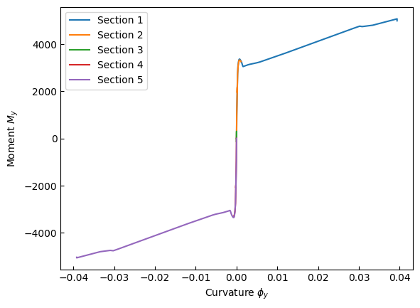
secDofs <U2 8B 'MY'[15]:
for sec in frame1defo.secPoints.data:
    x = frame1defo.sel(secPoints=sec).data
    y = frame1fo.sel(secPoints=sec).data
    plt.plot(x, y, label=f"Section {sec}")
plt.xlabel("Curvature $\\phi_y$")
plt.ylabel("Moment $M_y$")
plt.legend()
plt.show()