Eigen (Pyvista)

The eigenvalue (modal) visualization provides insights into the dynamic characteristics of the structure. It includes the following features:

• Mode Shapes: Visual representation of how the structure deforms under specific vibration modes.

• Natural Frequencies or Periods: Display of corresponding frequencies or periods for each mode, enabling detailed analysis of structural dynamics.

• Animation: Dynamic visualization of the mode shapes to better understand the structural response.

Using the visualization tools, you can:

1. Analyze the vibration patterns of the structure.

2. Identify critical modes that may impact structural performance.

3. Evaluate the effectiveness of design modifications in improving dynamic behavior.

import opstool as opst
import opstool.vis.pyvista as opsvis

Here, we use a built-in example from opstool, which is an example of a suspension bridge model primarily composed of frame elements and shell elements.

opst.load_ops_examples("SuspensionBridge")
# or your model code here

Save the eigen analysis results

Although not mandatory, you can use the save_eigen_data function to save eigenvalue analysis data, which can help you better understand how opstool operates.

Parameters:

• odb_tag: Specifies the label for the output database.

• mode_tag: Specifies the number of modes to save. Modal data within the range [1, mode_tag] will be saved.

For detailed usage, please refer to the opstool.post.save_eigen_data().

opst.post.save_eigen_data(odb_tag=1, mode_tag=10)

Using DomainModalProperties - Developed by: Massimo Petracca, Guido Camata, ASDEA Software Technology

OPSTOOL ::  Eigen data has been saved to .opstool.output/EigenData-1.nc!

modal visualization

The modal visualization feature allows you to explore the dynamic behavior of structures by visualizing their mode shapes.

Parameters:

• ``odb_tag``: Helps identify which database to read the results from.

• ``subplots``: When set to True, uses subplots to display multiple mode shapes in a single figure.

• ``mode_tags``: Specifies the modes to visualize.

  • For example, mode_tags=4 visualizes modes [1, 4].

  • mode_tags=[2, 5] visualizes modes from 2 to 5.

Note

The highest mode number specified in mode_tags must not exceed the maximum mode number saved using the save_eigen_data function.This flexibility allows for detailed and customized visualization of the modal data, making it easier to analyze structural behavior.

In actual use, notebook=False should be used. This is just for the convenience of generating documents.

opsvis.set_plot_props(point_size=0, line_width=3, cmap="coolwarm", notebook=True)

Note

If you are not working in Jupyter Notebook or JupyterLab, ensure that `notebook=False`.

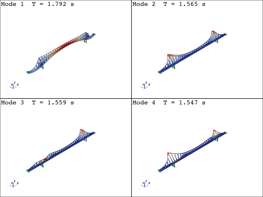
Plot mode shape by subplots

For detailed parameters and customization options, please refer to the opstool.vis.plotly.plot_eigen().

plotter = opsvis.plot_eigen(
    mode_tags=4,
    odb_tag=1,
    subplots=True,
)
plotter.show(jupyter_backend="jupyterlab")
# plotter.show()

OPSTOOL ::  Loading eigen data from .opstool.output/EigenData-1.nc ...

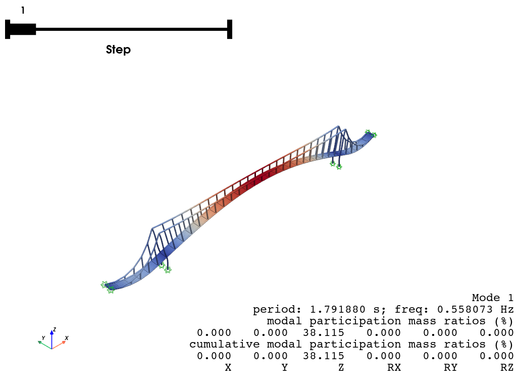
Plot mode shape by slides

When subplots set to False, displays the mode shapes as a slideshow, transitioning between modes.

plotter = opsvis.plot_eigen(
    mode_tags=3,
    odb_tag=1,
    subplots=False,
)
plotter.show(jupyter_backend="jupyterlab")
# plotter.show()

OPSTOOL ::  Loading eigen data from .opstool.output/EigenData-1.nc ...

Plot mode shape by animation

The following example demonstrates how to animate Mode 1:

plotter = opsvis.plot_eigen_animation(mode_tag=1, odb_tag=1, savefig="images/EigenAnimation.gif")
plotter.close()  # must be invoked to generate the gif
# plotter.show()

OPSTOOL ::  Loading eigen data from .opstool.output/EigenData-1.nc ...

Animation has been saved to images/EigenAnimation.gif!