Quickly apply gravity loads and obtain mass and stiffness matrices

This document mainly introduces some model data retrieval methods in opstool.

import matplotlib.pyplot as plt
import openseespy.opensees as ops

import opstool as opst
import opstool.vis.pyvista as opsvis

opsvis.set_plot_props(notebook=True)  # set notebook mode, you can set it to False for a practical use

Model

We will use two methods to add mass to the model: one is to specify the mass of the nodes using mass, and the other is to specify the linear density (-mass) when creating beam elements.

ops.wipe()
ops.model("basic", "-ndm", 2, "-ndf", 3)

# Define the model nodes
ops.node(1, 0.0, 0.0)
ops.node(2, 2.0, 0.0)
ops.node(3, 0.0, 2.0)
ops.node(4, 0.0, 2.0)
ops.node(5, 2.0, 2.0)
ops.node(6, 2.0, 2.0)

# Constrain the nodes
ops.rigidLink("beam", 3, 4)  # Rigid link between nodes 3 and 4
ops.equalDOF(5, 6, 1, 2, 3)  # Equal DOF between nodes 5 and 6

ops.fix(1, 1, 1, 1)
ops.fix(2, 1, 1, 1)

# Assign the node masses
ops.mass(1, 1.0, 1.0, 0.0)
ops.mass(2, 1.0, 1.0, 0.0)
ops.mass(3, 1.0, 1.0, 0.0)
ops.mass(4, 1.0, 1.0, 0.0)
ops.mass(5, 10.0, 10.0, 1e-3)
ops.mass(6, 10.0, 10.0, 1e-3)

# Define the elements
ops.geomTransf("Linear", 1)

# element('elasticBeamColumn', eleTag, *eleNodes, Area, E_mod, Iz, transfTag, <'-mass', mass>)
Area, E_mod, Iz = 1.0, 1.0, 1.0
ops.element("elasticBeamColumn", 1, 1, 3, Area, E_mod, Iz, 1, "-mass", 1.0)
ops.element("elasticBeamColumn", 2, 2, 5, Area, E_mod, Iz, 1, "-mass", 1.0)
ops.element("elasticBeamColumn", 3, 4, 6, Area, E_mod, Iz, 1, "-mass", 1.0)

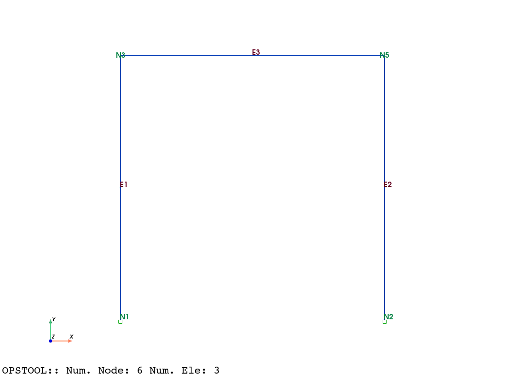
fig = opsvis.plot_model(show_node_numbering=True, show_ele_numbering=True)
fig.show(jupyter_backend="static")

Apply the gravity load

The opstool utility provides a function opstool.pre.create_gravity_load() to quickly apply gravity loads. This function internally retrieves all masses in the model, including those defined at nodes, in elements, and in materials. You only need to provide the multiplier (gravitational acceleration) and the direction of load application.

ops.timeSeries("Constant", 1)  # Define a constant time series, tag = 1
ops.pattern("Plain", 1, 1)  # Define a load pattern, tag = 1
node_loads = opst.pre.create_gravity_load(direction="Y", factor=-9.81)  # Create gravity loads in the pattern tag=1

A internally calls the load command to add node loads and also returns a dictionary of load values:

print("Node Loads:")
for node, load in node_loads.items():
    print(f"Node {node}: {load}")

Node Loads:
Node 1: [0.0, -19.62, 0.0]
Node 2: [0.0, -19.62, 0.0]
Node 3: [0.0, -19.62, 0.0]
Node 4: [0.0, -19.62, 0.0]
Node 5: [0.0, -107.91000000000001, 0.0]
Node 6: [0.0, -107.91000000000001, 0.0]

🤖 Therefore, you can easily create gravity loads directly through the above commands. The way you specify the mass when modeling is arbitrary. opstool can help you do all the internal conversions!

Get Model Mass

get_node_mass returns a dictionary containing all masses defined in the model, both at nodes and elements.

node_mass = opst.pre.get_node_mass()  # get the node mass dict

print("Node Masses:")
for node, mass in node_mass.items():
    print(f"Node {node}: {mass}")

Node Masses:
Node 1: [2.0, 2.0, 0.0]
Node 2: [2.0, 2.0, 0.0]
Node 3: [2.0, 2.0, 0.0]
Node 4: [2.0, 2.0, 0.0]
Node 5: [11.0, 11.0, 0.001]
Node 6: [11.0, 11.0, 0.001]

─── ⋆⋅☆⋅⋆ ── ✍️

▶️ First, part of it comes from

ops.mass(1, 1.0, 1.0, 0.0)
ops.mass(2, 1.0, 1.0, 0.0)
ops.mass(3, 1.0, 1.0, 0.0)
ops.mass(4, 1.0, 1.0, 0.0)
ops.mass(5, 10.0, 10.0, 1e-3)
ops.mass(6, 10.0, 10.0, 1e-3)

▶️ The second comes from the beam elements:

length = 2, density = 1.0, area = 1.0

The mass assigned to each node is:

length * density * area / 2 = 1.0

Therefore, the returned mass is completely accurate.

In practice, create_gravity_load calls get_node_mass to iteratively create nodal loads internally.

Get system matrix

You can get the mass, stiffness and damping matrix

Get Matrix from Penalty-constraint method

constraints_args = ["Penalty", 1e10, 1e10]  # This affects the dimensions of the matrix
system_args = ["FullGeneral"]  # Full matrix system must be used
numberer_args = ["RCM"]  # It affects the topology of the matrix and the order of dof.

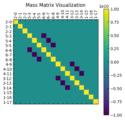
M = opst.pre.get_mck("m", constraints_args=constraints_args, system_args=system_args, numberer_args=numberer_args)
print("Mass Matrix shape:", M)
nodeTagsDofs1 = M.coords["nodeTagsDofs-1"].values  # "nodeTag-Dof" coordinate
nodeTagsDofs2 = M.coords["nodeTagsDofs-2"].values
M = M.values

Mass Matrix shape: <xarray.DataArray (nodeTagsDofs-1: 18, nodeTagsDofs-2: 18)> Size: 3kB
array([[ 1.e+10,  0.e+00,  0.e+00,  0.e+00,  0.e+00,  0.e+00,  0.e+00,
         0.e+00,  0.e+00,  0.e+00,  0.e+00,  0.e+00,  0.e+00,  0.e+00,
         0.e+00,  0.e+00,  0.e+00,  0.e+00],
       [ 0.e+00,  1.e+10,  0.e+00,  0.e+00,  0.e+00,  0.e+00,  0.e+00,
         0.e+00,  0.e+00,  0.e+00,  0.e+00,  0.e+00,  0.e+00,  0.e+00,
         0.e+00,  0.e+00,  0.e+00,  0.e+00],
       [ 0.e+00,  0.e+00,  1.e+10,  0.e+00,  0.e+00,  0.e+00,  0.e+00,
         0.e+00,  0.e+00,  0.e+00,  0.e+00,  0.e+00,  0.e+00,  0.e+00,
         0.e+00,  0.e+00,  0.e+00,  0.e+00],
       [ 0.e+00,  0.e+00,  0.e+00,  1.e+10,  0.e+00,  0.e+00, -1.e+10,
         0.e+00,  0.e+00,  0.e+00,  0.e+00,  0.e+00,  0.e+00,  0.e+00,
         0.e+00,  0.e+00,  0.e+00,  0.e+00],
       [ 0.e+00,  0.e+00,  0.e+00,  0.e+00,  1.e+10,  0.e+00,  0.e+00,
        -1.e+10,  0.e+00,  0.e+00,  0.e+00,  0.e+00,  0.e+00,  0.e+00,
         0.e+00,  0.e+00,  0.e+00,  0.e+00],
       [ 0.e+00,  0.e+00,  0.e+00,  0.e+00,  0.e+00,  1.e+10,  0.e+00,
         0.e+00, -1.e+10,  0.e+00,  0.e+00,  0.e+00,  0.e+00,  0.e+00,
         0.e+00,  0.e+00,  0.e+00,  0.e+00],
       [ 0.e+00,  0.e+00,  0.e+00, -1.e+10,  0.e+00,  0.e+00,  1.e+10,
         0.e+00,  0.e+00,  0.e+00,  0.e+00,  0.e+00,  0.e+00,  0.e+00,
...
         0.e+00,  0.e+00,  0.e+00,  0.e+00,  1.e+10,  0.e+00,  0.e+00,
        -1.e+10,  0.e+00,  0.e+00,  0.e+00],
       [ 0.e+00,  0.e+00,  0.e+00,  0.e+00,  0.e+00,  0.e+00,  0.e+00,
         0.e+00,  0.e+00, -1.e+10,  0.e+00,  0.e+00,  1.e+10,  0.e+00,
         0.e+00,  0.e+00,  0.e+00,  0.e+00],
       [ 0.e+00,  0.e+00,  0.e+00,  0.e+00,  0.e+00,  0.e+00,  0.e+00,
         0.e+00,  0.e+00,  0.e+00, -1.e+10,  0.e+00,  0.e+00,  1.e+10,
         0.e+00,  0.e+00,  0.e+00,  0.e+00],
       [ 0.e+00,  0.e+00,  0.e+00,  0.e+00,  0.e+00,  0.e+00,  0.e+00,
         0.e+00,  0.e+00,  0.e+00,  0.e+00, -1.e+10,  0.e+00,  0.e+00,
         1.e+10,  0.e+00,  0.e+00,  0.e+00],
       [ 0.e+00,  0.e+00,  0.e+00,  0.e+00,  0.e+00,  0.e+00,  0.e+00,
         0.e+00,  0.e+00,  0.e+00,  0.e+00,  0.e+00,  0.e+00,  0.e+00,
         0.e+00,  1.e+10,  0.e+00,  0.e+00],
       [ 0.e+00,  0.e+00,  0.e+00,  0.e+00,  0.e+00,  0.e+00,  0.e+00,
         0.e+00,  0.e+00,  0.e+00,  0.e+00,  0.e+00,  0.e+00,  0.e+00,
         0.e+00,  0.e+00,  1.e+10,  0.e+00],
       [ 0.e+00,  0.e+00,  0.e+00,  0.e+00,  0.e+00,  0.e+00,  0.e+00,
         0.e+00,  0.e+00,  0.e+00,  0.e+00,  0.e+00,  0.e+00,  0.e+00,
         0.e+00,  0.e+00,  0.e+00,  1.e+10]])
Coordinates:
  * nodeTagsDofs-1  (nodeTagsDofs-1) <U4 288B '2-0' '2-1' ... '1-16' '1-17'
  * nodeTagsDofs-2  (nodeTagsDofs-2) <U4 288B '2-0' '2-1' ... '1-16' '1-17'

plt.matshow(M, cmap="viridis")
plt.xticks(ticks=range(len(nodeTagsDofs1)), labels=nodeTagsDofs1, rotation=90)
plt.yticks(ticks=range(len(nodeTagsDofs2)), labels=nodeTagsDofs2)
plt.colorbar()
plt.title("Mass Matrix Visualization")
plt.show()

K = opst.pre.get_mck("k", constraints_args=constraints_args, system_args=system_args, numberer_args=numberer_args)
K = K.values
print("Stiffness Matrix (K):")
print(K.shape)

Stiffness Matrix (K):
(18, 18)

plt.matshow(K, cmap="viridis")
plt.xticks(ticks=range(len(nodeTagsDofs1)), labels=nodeTagsDofs1, rotation=90)
plt.yticks(ticks=range(len(nodeTagsDofs2)), labels=nodeTagsDofs2)
plt.colorbar()
plt.title("Stiffness Matrix Visualization")
plt.show()

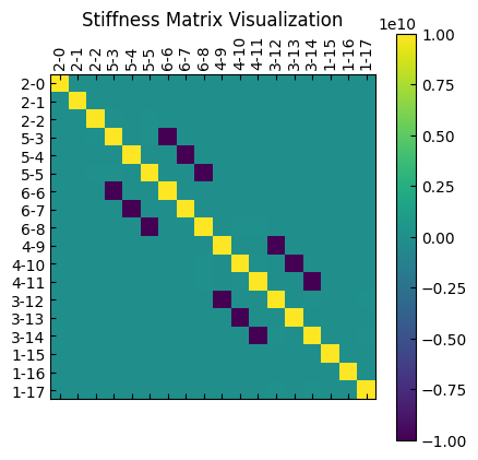
It can be observed that all degrees of freedom are preserved in the system matrix, and a large penalty number is added.

Get Matrix from Transformation-constraint approach

constraints_args = ["Transformation"]  # This affects the dimensions of the matrix
system_args = ["FullGeneral"]  # Full matrix system must be used
numberer_args = ["Plain"]  # It affects the topology of the matrix and the order of dof.

K = opst.pre.get_mck("k", constraints_args=constraints_args, system_args=system_args, numberer_args=numberer_args)
nodeTagsDofs1 = K.coords["nodeTagsDofs-1"].values  # "nodeTag-Dof" coordinate
nodeTagsDofs2 = K.coords["nodeTagsDofs-2"].values
K = K.values
print("Stiffness Matrix (K):")
print(K)

Stiffness Matrix (K):
[[ 2.   0.   1.5 -0.5  0.   0. ]
 [ 0.   2.   1.5  0.  -1.5  1.5]
 [ 1.5  1.5  4.   0.  -1.5  1. ]
 [-0.5  0.   0.   2.   0.   1.5]
 [ 0.  -1.5 -1.5  0.   2.  -1.5]
 [ 0.   1.5  1.   1.5 -1.5  4. ]]

plt.matshow(K, cmap="viridis")
plt.xticks(ticks=range(len(nodeTagsDofs1)), labels=nodeTagsDofs1, rotation=90)
plt.yticks(ticks=range(len(nodeTagsDofs2)), labels=nodeTagsDofs2)
plt.colorbar()
plt.title("Stiffness Matrix Visualization")
plt.show()

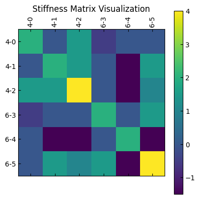
It can be observed that the constrained degrees of freedom are eliminated from the system matrix (only nodes 4 and 6 are retained), thus reducing the dimension of the system matrix.