Post-processing for fiber section responses
This example is adapted from:
Reinforced Concrete Frame Pushover Analysis
Note
Since fiber cross-sections typically have a large number of fiber points, it is not recommended to save the responses of all elements when the number of elements is large. It is recommended to save only the responses of critical elements.
[1]:
import matplotlib.pyplot as plt
import numpy as np
import openseespy.opensees as ops

import opstool as opst
Model
[2]:
ops.wipe()
ops.model("basic", "-ndm", 3, "-ndf", 6)
width = 360.0
height = 144.0
ops.node(1, 0.0, 0.0, 0.0)
ops.node(2, width, 0.0, 0.0)
ops.node(3, 0.0, 0.0, height)
ops.node(4, width, 0.0, height)
ops.fix(1, 1, 1, 1, 1, 1, 1)
ops.fix(2, 1, 1, 1, 1, 1, 1)

matTagConc1 = 1  # CORE
matTagConc2 = 2  # COVER
ops.uniaxialMaterial("Concrete02", matTagConc1, -6.0, -0.004, -5.0, -0.014, 0.2, 0.6, 300)
ops.uniaxialMaterial("Concrete02", matTagConc2, -5.0, -0.002, 0.0, -0.006, 0.2, 0.6, 300)

fy = 60.0
E = 30000.0
matTagSteel = 3
ops.uniaxialMaterial("Steel01", matTagSteel, fy, E, 0.01)
[3]:
colWidth = 15
colDepth = 24
cover = 1.5
As = 0.60 # area of no. 7 bars
dia = 2 * np.sqrt(As / np.pi)
y1 = colDepth / 2.0
z1 = colWidth / 2.0
outer_points = [(-y1, -z1), (y1, -z1), (y1, z1), (-y1, z1)]
inner_points = opst.pre.section.offset(outer_points, d=cover)
cover_patch = opst.pre.section.create_polygon_patch(outer_points, holes=[inner_points])
core_patch = opst.pre.section.create_polygon_patch(inner_points)
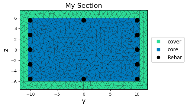
SEC = opst.pre.section.SecMesh()
SEC.add_patch_group({"cover": cover_patch, "core": core_patch})
SEC.set_ops_mat_tag({"cover": matTagConc2, "core": matTagConc1})
SEC.set_mesh_size(1)
SEC.add_rebar_line(
points=[(y1 - cover - dia / 2, z1 - cover - dia / 2), (y1 - cover - dia / 2, cover - z1 + dia / 2)],
n=5,
dia=dia,
ops_mat_tag=matTagSteel,
)
SEC.add_rebar_line(
points=[(0.0, z1 - cover - dia / 2), (0.0, cover - z1 + dia / 2)], n=2, dia=dia, ops_mat_tag=matTagSteel
)
SEC.add_rebar_line(
points=[(cover - y1 + dia / 2, z1 - cover - dia / 2), (cover - y1 + dia / 2, cover - z1 + dia / 2)],
n=5,
dia=dia,
ops_mat_tag=matTagSteel,
)
SEC.mesh()
ax = SEC.view()
plt.show()
OPSTOOL™ :: The section My Section has been successfully meshed!
We can save this section class:
[4]:
import pickle

with open("data/my-section.pkl", "wb") as f:
    pickle.dump(SEC, f)
[5]:
SEC.to_opspy_cmds(secTag=1, GJ=1000000)  # to OpenSeesPy commands

# Define column elements
# ----------------------
ops.geomTransf("PDelta", 1, -1, 0, 0)
# Number of integration points along length of element
np_ = 5
# Lobatto integratoin
ops.beamIntegration("Lobatto", 1, 1, np_)
eleType = "forceBeamColumn"
ops.element(eleType, 1, 1, 3, 1, 1)
ops.element(eleType, 2, 2, 4, 1, 1)

# Define beam elment
# -----------------------------
ops.geomTransf("Linear", 2, 0.0, 0.0, 1.0)
ops.element("elasticBeamColumn", 3, 3, 4, 360.0, 4030.0, 2015.0, 10000, 8640.0, 8640.0, 2)
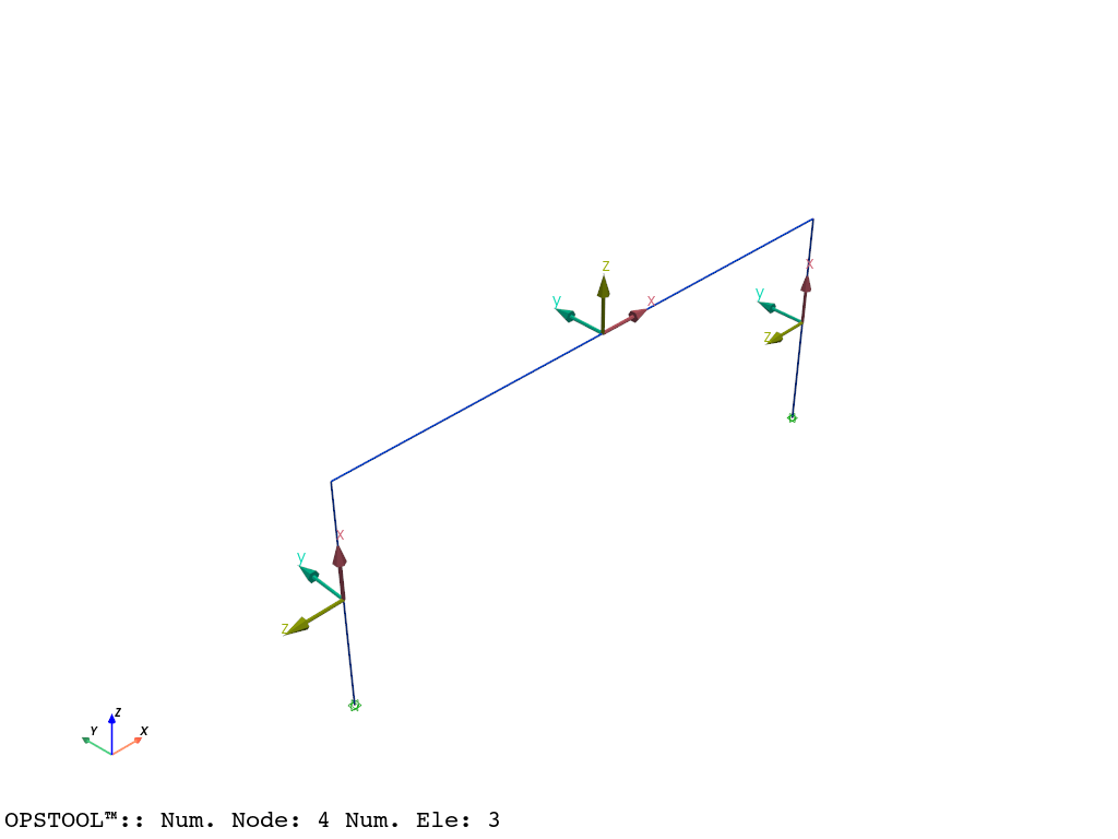
[6]:
opst.vis.pyvista.set_plot_props(notebook=True)  # you should not use
fig = opst.vis.pyvista.plot_model(show_local_axes=True)
fig.show(jupyter_backend="jupyterlab")
# fig.show()
Gravity analysis
[7]:
# Define gravity loads
# --------------------

#  a parameter for the axial load
P = 180.0  # 10% of axial capacity of columns

# Create a Plain load pattern with a Linear TimeSeries
ops.timeSeries("Linear", 1)
ops.pattern("Plain", 1, 1)

# Create nodal loads at nodes 3 & 4
#    nd  FX,  FY, MZ
ops.load(3, 0.0, 0.0, -P, 0.0, 0.0, 0.0)
ops.load(4, 0.0, 0.0, -P, 0.0, 0.0, 0.0)

# Start of analysis generation
# ------------------------------
ops.system("BandGeneral")
ops.constraints("Transformation")
ops.numberer("RCM")
ops.test("NormDispIncr", 1.0e-12, 10, 3)
ops.algorithm("Newton")
ops.integrator("LoadControl", 0.1)
ops.analysis("Static")
ops.analyze(10)
[7]:
0
Pushover analysis
Define lateral loads
[8]:
ops.loadConst("-time", 0.0)
# Define lateral loads
# --------------------
# Set some parameters
H = 10.0  # Reference lateral load
# Set lateral load pattern with a Linear TimeSeries
ops.pattern("Plain", 2, 1)
ops.load(3, H, 0.0, 0.0, 0.0, 0.0, 0.0)
ops.load(4, H, 0.0, 0.0, 0.0, 0.0, 0.0)
Start of modifications to analysis for push over
[9]:
# Set some parameters
dU = 0.1  # Displacement increment
ops.integrator("DisplacementControl", 3, 1, dU)
# Set some parameters
maxU = 15.0  # Max displacement
currentDisp = 0.0
ok = 0

ops.test("NormDispIncr", 1.0e-6, 1000)
ops.algorithm("KrylovNewton")
Save the responses. Args see CreateODB
[10]:
ODB = opst.post.CreateODB(odb_tag=1, save_fiber_sec_resp=True, fiber_ele_tags=[1, 2])
while ok == 0 and currentDisp < maxU:
    ok = ops.analyze(1)

    # if the analysis fails try initial tangent iteration
    if ok != 0:
        print("KrylovNewton failed")
        break

    ODB.fetch_response_step()

    currentDisp = ops.nodeDisp(3, 1)

ODB.save_response()
OPSTOOL™ ::  All responses data with _odb_tag = 1 saved in
g:\opstool\docs\src\post\.opstool.output\RespStepData-1.odb!
Post-processing
[11]:
info = opst.post.get_element_responses_info(ele_type="FiberSection")
ele_type: FiberSection
Available Response Types (resp_type):
  - Stresses
    resp_dim: ['time', 'eleTags', 'secPoints', 'fiberPoints']
    resp_dof: None
  - Strains
    resp_dim: ['time', 'eleTags', 'secPoints', 'fiberPoints']
    resp_dof: None
  - secForce
    resp_dim: ['time', 'eleTags', 'secPoints', 'DOFs']
    resp_dof: ['P', 'Mz', 'My', 'T']
  - secDefo
    resp_dim: ['time', 'eleTags', 'secPoints', 'DOFs']
    resp_dof: ['P', 'Mz', 'My', 'T']
Fiber Section
Extracting fiber cross responses
[12]:
sec_resp = opst.post.get_element_responses(odb_tag=1, ele_type="FiberSection")  # odb_tag=1 as above
print(sec_resp.data_vars)
print("-" * 100)
print(sec_resp.dims)
print("-" * 100)
print(sec_resp.coords)
OPSTOOL™ ::  Loading FiberSection response data from g:\opstool\docs\src\post\.opstool.output\RespStepData-1.odb
...
Data variables:
    areas     (eleTags, secPoints, fiberPoints) float64 90kB 0.3809 ... 0.6
    matTags   (eleTags, secPoints, fiberPoints) float64 90kB 2.0 2.0 ... 3.0 3.0
    secDefo   (time, eleTags, secPoints, DOFs) float32 24kB -0.0001213 ... 1....
    secForce  (time, eleTags, secPoints, DOFs) float32 24kB -180.0 ... 0.1157
    Strains   (time, eleTags, secPoints, fiberPoints) float32 7MB -0.0001213 ...
    Stresses  (time, eleTags, secPoints, fiberPoints) float32 7MB -0.588 ... ...
    ys        (eleTags, secPoints, fiberPoints) float64 90kB -11.73 ... -10.06
    zs        (eleTags, secPoints, fiberPoints) float64 90kB 3.354 ... -5.563
----------------------------------------------------------------------------------------------------
FrozenMappingWarningOnValuesAccess({'eleTags': 2, 'secPoints': 5, 'fiberPoints': 1129, 'time': 152, 'DOFs': 4})
----------------------------------------------------------------------------------------------------
Coordinates:
  * eleTags      (eleTags) int64 16B 1 2
  * secPoints    (secPoints) int64 40B 1 2 3 4 5
  * fiberPoints  (fiberPoints) int64 9kB 1 2 3 4 5 ... 1125 1126 1127 1128 1129
  * time         (time) float32 608B 0.0 0.6684 1.319 ... 3.097 3.091 3.086
  * DOFs         (DOFs) <U2 32B 'P' 'Mz' 'My' 'T'
We can select the responses of element 1 and its first section, time=-1 means that the last time is used.
[13]:
stress = sec_resp["Stresses"].sel(eleTags=1, secPoints=1).isel(time=-1)
strain = sec_resp["Strains"].sel(eleTags=1, secPoints=1).isel(time=-1)
y = sec_resp["ys"].sel(eleTags=1, secPoints=1)
z = sec_resp["zs"].sel(eleTags=1, secPoints=1)
points = np.stack((y.values, z.values), axis=-1)  # (num_fiber_points, 2), used for plotting response
print("-" * 100)
print("strain\n", strain.coords)  # eleTags, time, secPoints are fixed by sel and isel above, fiberPoints remain
print("-" * 100)
print("y\n", y.coords)  # eleTags, secPoints are fixed by sel and isel above, fiberPoints remain
print("-" * 100)
print("points\n", points.shape)  # (num_fiber_points, 2)
----------------------------------------------------------------------------------------------------
strain
 Coordinates:
  * fiberPoints  (fiberPoints) int64 9kB 1 2 3 4 5 ... 1125 1126 1127 1128 1129
    eleTags      int64 8B 1
    secPoints    int64 8B 1
    time         float32 4B 3.086
----------------------------------------------------------------------------------------------------
y
 Coordinates:
  * fiberPoints  (fiberPoints) int64 9kB 1 2 3 4 5 ... 1125 1126 1127 1128 1129
    eleTags      int64 8B 1
    secPoints    int64 8B 1
----------------------------------------------------------------------------------------------------
points
 (1129, 2)
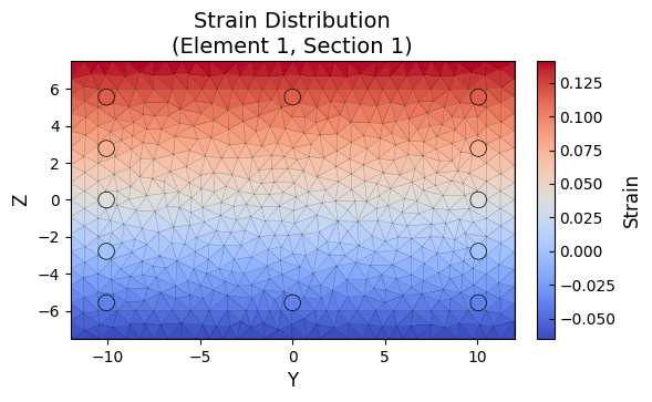
Plotting the strain distribution:
In version v1.0.21 and later, the SecMesh class added a function plot_response to visualize a given response, which automatically maps the response based on the coordinates of the triangular mesh.
[14]:
import pickle

with open("data/my-section.pkl", "rb") as f:
    SEC = pickle.load(f)
[15]:
fig, ax = plt.subplots(figsize=(6, 5))
ax, cbar = SEC.plot_response(
    points=points,  # (num_fiber_points, 2)
    response=strain,  # (num_fiber_points,)
    mat_tag=None,
    cmap="coolwarm",
    ax=ax,
)
cbar.set_label("Strain", fontsize=12)
ax.set_title("Strain Distribution\n(Element 1, Section 1)", fontsize=14)
ax.set_xlabel("Y", fontsize=12)
ax.set_ylabel("Z", fontsize=12)
fig.tight_layout(rect=[0, 0, 1, 1])

plt.show()
We can also use imageio to create animations for all moments.
Here, we select concrete fibers (material tag with 1 and 2) using Boolean operations, and then specify a failure threshold for these two materials using a threshold parameter. Mesh elements exceeding the threshold are hollowed out to simulate failure.
[16]:
import imageio.v2 as imageio

mat = sec_resp["matTags"].sel(eleTags=1, secPoints=1)
cond = (mat == 1) | (mat == 2)  # concrete fibers only
# overall min strain across all time steps
vmin = sec_resp["Strains"].sel(eleTags=1, secPoints=1, fiberPoints=cond).min().values
# overall max strain across all time steps
vmax = sec_resp["Strains"].sel(eleTags=1, secPoints=1, fiberPoints=cond).max().values

with imageio.get_writer("images/fiber-section-strain.gif", mode="I", fps=6) as writer:
    for t in range(len(sec_resp["time"])):
        strain = sec_resp["Strains"].sel(eleTags=1, secPoints=1).isel(time=t)

        fig, ax = plt.subplots(figsize=(6, 5))
        ax, cbar = SEC.plot_response(
            points=points,
            response=strain.values,
            cmap="Spectral_r",
            ax=ax,
            mat_tag=[1, 2],  # concrete fibers only
            thresholds={2: (-0.006, 0.002), 1: (-0.015, 0.002)},  # failure thresholds, 2: cover, 1: core
        )
        cbar.set_label("Strain", fontsize=12)
        cbar.mappable.set_clim(vmin, vmax)
        ax.set_title("Strain Distribution\n(Element 1, Section 1)", fontsize=14)
        ax.set_xlabel("Y", fontsize=12)
        ax.set_ylabel("Z", fontsize=12)
        fig.tight_layout(rect=[0, 0, 1, 1])

        # Convert Matplotlib figure to image and append to gif
        fig.canvas.draw()
        image = np.frombuffer(fig.canvas.buffer_rgba(), dtype=np.uint8)
        image = image.reshape((*fig.canvas.get_width_height()[::-1], 4))
        writer.append_data(image)

        plt.close(fig)
Similarly, we can also visualize stress.
[17]:
mat = sec_resp["matTags"].sel(eleTags=1, secPoints=1)
cond = (mat == 1) | (mat == 2)  # concrete fibers only
vmin = sec_resp["Stresses"].sel(eleTags=1, secPoints=1, fiberPoints=cond).min().values
vmax = sec_resp["Stresses"].sel(eleTags=1, secPoints=1, fiberPoints=cond).max().values

with imageio.get_writer("images/fiber-section-stress.gif", mode="I", fps=5) as writer:
    for t in range(len(sec_resp["time"])):
        stress = sec_resp["Stresses"].sel(eleTags=1, secPoints=1).isel(time=t)

        fig, ax = plt.subplots(figsize=(6, 5))
        ax, cbar = SEC.plot_response(points=points, response=stress, mat_tag=[1, 2], cmap="jet", ax=ax)
        cbar.set_label("Stress", fontsize=12)
        cbar.mappable.set_clim(vmin, vmax)
        ax.set_title("Concrete Stress Distribution\n(Element 1, Section 1)", fontsize=14)
        ax.set_xlabel("Y", fontsize=12)
        ax.set_ylabel("Z", fontsize=12)
        fig.tight_layout(rect=[0, 0, 1, 1])

        fig.canvas.draw()
        image = np.frombuffer(fig.canvas.buffer_rgba(), dtype=np.uint8)
        image = image.reshape((*fig.canvas.get_width_height()[::-1], 4))
        writer.append_data(image)

        plt.close(fig)
Of course, we can also handle it ourselves.
[18]:
# We can also extract stresses and strains for specific materials.
stress = sec_resp["Stresses"].sel(eleTags=1, secPoints=1).isel(time=-1)
strain = sec_resp["Strains"].sel(eleTags=1, secPoints=1).isel(time=-1)
y = sec_resp["ys"].sel(eleTags=1, secPoints=1)
z = sec_resp["zs"].sel(eleTags=1, secPoints=1)
mat = sec_resp["matTags"].sel(eleTags=1, secPoints=1)

cond = (mat == 1) | (mat == 2)
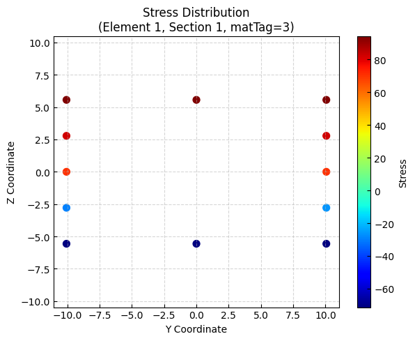
matTag = 3 for rebar:
[19]:
plt.figure(figsize=(6, 5))
scatter = plt.scatter(y[~cond], z[~cond], c=stress[~cond], cmap="jet", s=50)
plt.xlabel("Y Coordinate")
plt.ylabel("Z Coordinate")
plt.title("Stress Distribution\n(Element 1, Section 1, matTag=3)")
plt.colorbar(scatter, label="Stress")
plt.axis("equal")
plt.grid(True, linestyle="--", alpha=0.5)
plt.tight_layout()
plt.show()
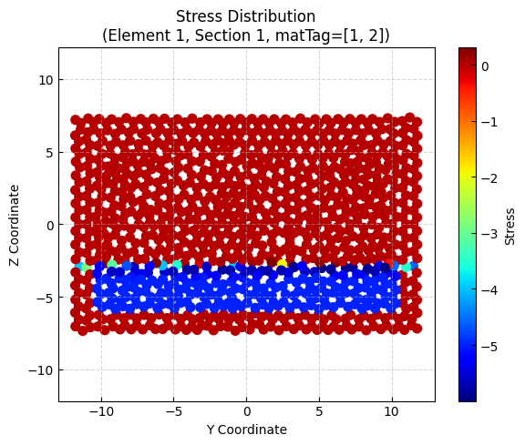
mattag = [1, 2] for concrete:
[20]:
plt.figure(figsize=(6, 5))
scatter = plt.scatter(y[cond], z[cond], c=stress[cond], cmap="jet", s=50)
plt.xlabel("Y Coordinate")
plt.ylabel("Z Coordinate")
plt.title("Stress Distribution\n(Element 1, Section 1, matTag=[1, 2])")
plt.colorbar(scatter, label="Stress")
plt.axis("equal")
plt.grid(True, linestyle="--", alpha=0.5)
plt.tight_layout()
plt.show()
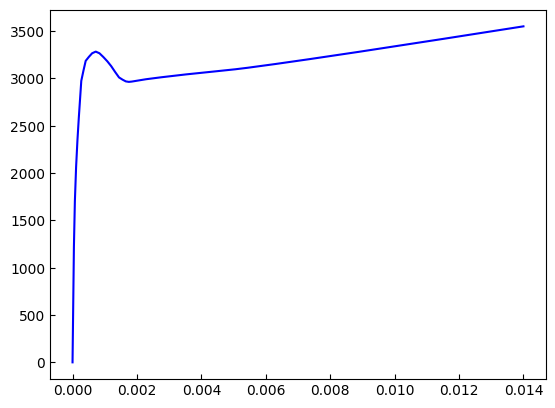
We can also extract the force and deformation response at the cross-section level
[21]:
defo = sec_resp["secDefo"].sel(eleTags=1, secPoints=1, DOFs="My")
fo = sec_resp["secForce"].sel(eleTags=1, secPoints=1, DOFs="My")
print(defo.head())
<xarray.DataArray 'secDefo' (time: 5)> Size: 20B
array([1.2732308e-21, 2.0417334e-05, 4.3028922e-05, 7.2857343e-05,
       1.1079801e-04], dtype=float32)
Coordinates:
  * time       (time) float32 20B 0.0 0.6684 1.319 1.874 2.323
    DOFs       <U2 8B 'My'
    eleTags    int64 8B 1
    secPoints  int64 8B 1
[22]:
plt.plot(defo, fo, c="b")
plt.show()
Frame elements
[23]:
frame_resp = opst.post.get_element_responses(odb_tag=1, ele_type="Frame")
print(frame_resp)
OPSTOOL™ :: Loading Frame response data from g:\opstool\docs\src\post\.opstool.output\RespStepData-1.odb ...
<xarray.DatasetView> Size: 260kB
Dimensions:              (time: 152, eleTags: 3, basicDofs: 6, localDofs: 12,
                          secPoints: 7, secDofs: 6, locs: 4)
Coordinates:
  * time                 (time) float32 608B 0.0 0.6684 1.319 ... 3.091 3.086
  * eleTags              (eleTags) int64 24B 1 2 3
  * basicDofs            (basicDofs) <U3 72B 'N' 'MZ1' 'MZ2' 'MY1' 'MY2' 'T'
  * localDofs            (localDofs) <U3 144B 'FX1' 'FY1' 'FZ1' ... 'MY2' 'MZ2'
  * secPoints            (secPoints) int64 56B 1 2 3 4 5 6 7
  * secDofs              (secDofs) <U2 48B 'N' 'MZ' 'VY' 'MY' 'VZ' 'T'
  * locs                 (locs) <U5 80B 'alpha' 'X' 'Y' 'Z'
Data variables:
    basicDeformations    (time, eleTags, basicDofs) float32 11kB -0.01746 ......
    basicForces          (time, eleTags, basicDofs) float32 11kB -180.0 ... -...
    localForces          (time, eleTags, localDofs) float32 22kB -180.0 ... -...
    plasticDeformation   (time, eleTags, basicDofs) float32 11kB -0.0003215 ....
    sectionDeformations  (time, eleTags, secPoints, secDofs) float32 77kB -0....
    sectionForces        (time, eleTags, secPoints, secDofs) float32 77kB -18...
    sectionLocs          (time, eleTags, secPoints, locs) float32 51kB 0.0 .....
Attributes:
    localDofs:  local coord system dofs at end 1 and end 2
    basicDofs:  basic coord system dofs at end 1 and end 2
    secPoints:  section points No.
    secDofs:    section forces and deformations Dofs. Note that the section D...
    Notes:      Note that the deformations are displacements and rotations in...
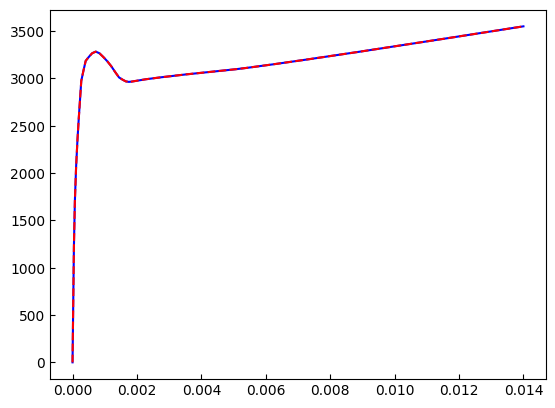
[24]:
fo2 = frame_resp["sectionForces"].sel(eleTags=1, secPoints=1, secDofs="MY")
defo2 = frame_resp["sectionDeformations"].sel(eleTags=1, secPoints=1, secDofs="MY")
[25]:
plt.plot(defo2, fo2, c="b")
plt.plot(defo, fo, "--r")
plt.show()
[26]:
fos = frame_resp["sectionForces"].sel(eleTags=1, secDofs="MY").isel(time=-1)
defos = frame_resp["sectionDeformations"].sel(eleTags=1, secDofs="MY").isel(time=-1)
[27]:
sec_loc = frame_resp["sectionLocs"].sel(eleTags=1)
xloc = sec_loc.sel(locs="X").isel(time=-1)
yloc = sec_loc.sel(locs="Y").isel(time=-1)
zloc = sec_loc.sel(locs="Z").isel(time=-1)
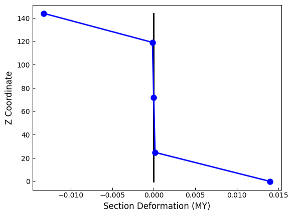
[28]:
plt.plot(xloc, zloc, "-k", lw=2)
plt.plot(xloc + defos, zloc, "-b", lw=2, marker="o", markersize=8)
plt.xlabel("Section Deformation (MY)", fontsize=12)
plt.ylabel("Z Coordinate", fontsize=12)
plt.show()