Note
Go to the end to download the full example code.
Double-Layer Shallow Dome
This is adapted from an example created by Amir Hossein Namadchi.
This is an OpenSeesPy simulation of one of the numerical examples in our previously published paper. The Core was purely written in Mathematica. This is my attempt to perform the analysis again via Opensees Core, to see if I can get the similar results. In the paper, we used Total Lagrangian framework to model the structure. Unfortunately, OpenSees does not include this framework, so, alternatively, I will use Corotational truss element.
import matplotlib.pyplot as plt
import numpy as np
import openseespy.opensees as ops

import opstool as opst
import opstool.vis.plotly as opsvis

# import opstool.vis.pyvista as opsvis
Below, the base units are defined as python variables:
## Units
m = 1  # Meters
KN = 1  # KiloNewtons
s = 1  # Seconds
Model Defintion
The coordinates information for each node are stored node_coords. Each row represent a node with the corresponding coordinates. Elements configuration are also described in connectivity, each row representing an element with its node IDs. Elements cross-sectional areas are stored in area_list. This appraoch, offers a more pythonic and flexible code when building the model. Since this is a relatively large model, some data will be read from external .txt files to keep the code cleaner.
# Node Coordinates Matrix (size : nn x 3)
node_coords = np.loadtxt("utils/DLSDome_nodes.txt", dtype=np.float64) * m

# Element Connectivity Matrix (size: nel x 2)
connectivity = np.loadtxt("utils/DLSDome_connectivity.txt", dtype=np.int64).tolist()

# Loaded Nodes
loaded_nodes = np.loadtxt("utils/DLSDome_loaded_nodes.txt", dtype=np.int64).tolist()

# Get Number of total Nodes
nn = len(node_coords)
# Get Number of total Elements
nel = len(connectivity)

# Cross-sectional area list (size: nel)
area_list = np.ones(nel) * (0.001) * (m**2)

# Modulus of Elasticity list (size: nel)
E_list = np.ones(nel) * (2.0 * 10**8) * (KN / m**2)

# Mass Density
rho = 7.850 * ((KN * s**2) / (m**4))

# Boundary Conditions (size: fixed_nodes x 4)
B_C = np.column_stack((np.arange(1, 31), np.ones((30, 3), dtype=np.int64))).tolist()
Model Construction
I use <i>list comprehension</i> to add nodes,elements and other objects to the domain.
ops.wipe()
ops.model("basic", "-ndm", 3, "-ndf", 3)

# Adding nodes to the model object using list comprehensions
[ops.node(n + 1, *node_coords[n]) for n in range(nn)]
# Applying BC
[ops.fix(B_C[n][0], *B_C[n][1:]) for n in range(len(B_C))]
# Set Material
ops.uniaxialMaterial("Elastic", 1, E_list[0])

# Adding Elements
[
    ops.element(
        "corotTruss",
        e + 1,
        *connectivity[e],
        area_list[e],
        1,
        "-rho",
        rho * area_list[e],
        "-cMass",
        1,
    )
    for e in range(nel)
]
print(f"Number of Nodes: {nn}, Number of Elements: {nel}")
Number of Nodes: 390, Number of Elements: 1410
Draw model
opsvis.set_plot_colors(truss="blue")
fig = opsvis.plot_model()
fig
# fig.show(renderer="browser")
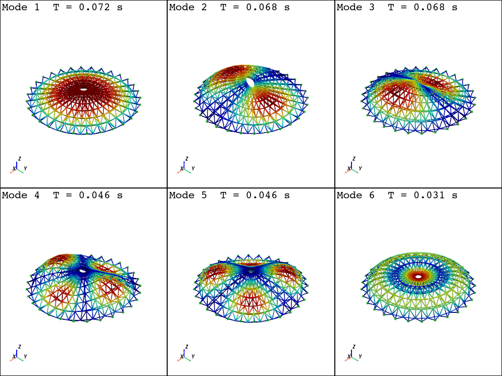
Eigenvalue Analysis
Let’s get the first 6 periods of the structure to see if they coincide with the ones in paper.
opst.post.save_eigen_data(odb_tag="eigen", mode_tag=6)
fig = opsvis.plot_eigen(odb_tag="eigen", mode_tags=6, subplots=True)
fig
# fig.show()
OPSTOOL™ ::  Eigen data has been saved to G:\opstool\docs\.opstool.output/EigenData-eigen.zarr!
OPSTOOL™ ::  Loading eigen data from G:\opstool\docs\.opstool.output/EigenData-eigen.zarr ...
fig = opst.vis.pyvista.plot_eigen(odb_tag="eigen", mode_tags=6, subplots=True)
fig.show()
OPSTOOL™ :: Loading eigen data from G:\opstool\docs\.opstool.output/EigenData-eigen.zarr ...
model_props, eigen_vectors = opst.post.get_eigen_data(odb_tag="eigen")

model_props_df = model_props.to_pandas()
model_props_df.head()
OPSTOOL™ :: Loading eigen data from G:\opstool\docs\.opstool.output/EigenData-eigen.zarr ...
print(f"*** Eigen periods:\n {model_props_df['eigenPeriod']}")
*** Eigen periods:
 modeTags
1    0.071892
2    0.068096
3    0.068096
4    0.046484
5    0.046484
6    0.031170
Name: eigenPeriod, dtype: float64
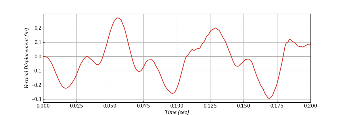
Dynamic Analysis
Great accordance is obtained in eigenvalue analysis. Now, let’s do wipeAnalysis() and perform dynamic analysis. The Newmark time integration algorithm with \(\gamma=0.5\) and \(\beta=0.25\) (Constant Average Acceleration Algorithm) is used. Harmonic loads are applied vertically on the loaded_nodes nodes.
ops.wipeAnalysis()


# define load function
def P(t):
    """Load function"""
    return 250 * np.sin(250 * t)


# Dynamic Analysis Parameters
dt = 0.00025
time = 0.2
time_domain = np.arange(0, time, dt)

# Adding loads to the domain beautifully
ops.timeSeries(
    "Path",
    1,
    "-dt",
    dt,
    "-values",
    *np.vectorize(P)(time_domain),
    "-time",
    *time_domain,
)
ops.pattern("Plain", 1, 1)
[ops.load(n, *[0, 0, -1]) for n in loaded_nodes]
# Analysis
ops.constraints("Plain")
ops.numberer("Plain")
ops.system("ProfileSPD")
ops.test("NormUnbalance", 0.0000001, 100)
ops.algorithm("ModifiedNewton")
ops.integrator("Newmark", 0.5, 0.25)
ops.analysis("Transient")
Save the results
ODB = opst.post.CreateODB(odb_tag=1)

for i in range(len(time_domain)):
    is_done = ops.analyze(1, dt)
    if is_done != 0:
        print("Failed to Converge!")
        break
    ODB.fetch_response_step()
ODB.save_response(zlib=True)  # for compressing the file
G:\opstool\examples\postprocessing\ex-double-layer-shallow-dome.py:175: DeprecationWarning:

The zlib parameter in save_response() is deprecated. Please set zlib in CreateODB().

OPSTOOL™ ::  All responses data with _odb_tag = 1 saved in G:\opstool\docs\.opstool.output\RespStepData-1.odb!
Visualization
Retrieving Nodal Response Results
node_resp = opst.post.get_nodal_responses(odb_tag=1)
print(node_resp.head())
OPSTOOL™ ::  Loading all response data from G:\opstool\docs\.opstool.output\RespStepData-1.odb ...
<xarray.Dataset> Size: 3kB
Dimensions:             (time: 5, nodeTags: 5, DOFs: 5)
Coordinates:
  * time                (time) float32 20B 0.0 0.00025 0.0005 0.00075 0.001
  * nodeTags            (nodeTags) int64 40B 1 2 3 4 5
  * DOFs                (DOFs) <U2 40B 'UX' 'UY' 'UZ' 'RX' 'RY'
Data variables:
    accel               (time, nodeTags, DOFs) float32 500B 0.0 0.0 ... 0.0 0.0
    disp                (time, nodeTags, DOFs) float32 500B 0.0 0.0 ... 0.0 0.0
    pressure            (time, nodeTags) float32 100B 0.0 0.0 0.0 ... 0.0 0.0
    rayleighForces      (time, nodeTags, DOFs) float32 500B 0.0 0.0 ... 0.0 0.0
    reaction            (time, nodeTags, DOFs) float32 500B 0.0 0.0 ... 0.0 0.0
    reactionIncInertia  (time, nodeTags, DOFs) float32 500B 0.0 0.0 ... 0.0 0.0
    vel                 (time, nodeTags, DOFs) float32 500B 0.0 0.0 ... 0.0 0.0
Attributes:
    UX:       Displacement in X direction
    UY:       Displacement in Y direction
    UZ:       Displacement in Z direction
    RX:       Rotation about X axis
    RY:       Rotation about Y axis
    RZ:       Rotation about Z axis
We select the target data through the indexing method provided by xarray.
time = node_resp["time"].values
disp = node_resp["disp"].sel(nodeTags=362, DOFs="UZ")
plt.figure(figsize=(12, 4))
plt.plot(time, disp, color="#d62d20", linewidth=1.75)
plt.ylabel(
    "Vertical Displacement (m)",
    {"fontname": "Cambria", "fontstyle": "italic", "size": 14},
)
plt.xlabel("Time (sec)", {"fontname": "Cambria", "fontstyle": "italic", "size": 14})
plt.xlim([0.0, max(time)])
plt.grid()
plt.yticks(fontname="Cambria", fontsize=14)
plt.xticks(fontname="Cambria", fontsize=14)
plt.show()
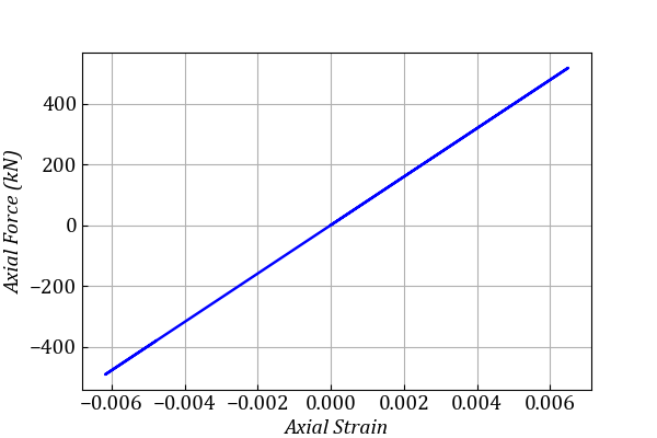
Retrieving Element Response Results
ele_resp = opst.post.get_element_responses(odb_tag=1, ele_type="Truss")
print(ele_resp.head())
OPSTOOL™ ::  Loading Truss response data from G:\opstool\docs\.opstool.output\RespStepData-1.odb ...
<xarray.Dataset> Size: 460B
Dimensions:     (time: 5, eleTags: 5)
Coordinates:
  * time        (time) float32 20B 0.0 0.00025 0.0005 0.00075 0.001
  * eleTags     (eleTags) int64 40B 1 2 3 4 5
Data variables:
    axialDefo   (time, eleTags) float32 100B 0.0 0.0 0.0 ... 2.955e-06 2.955e-06
    axialForce  (time, eleTags) float32 100B 0.0 0.0 0.0 ... 0.2356 0.2356
    Strain      (time, eleTags) float32 100B 0.0 0.0 0.0 ... 1.178e-06 1.178e-06
    Stress      (time, eleTags) float32 100B 0.0 0.0 0.0 ... 235.6 235.6 235.6
force = ele_resp["axialForce"].sel(eleTags=10)
defo = ele_resp["axialDefo"].sel(eleTags=10)
plt.figure(figsize=(6, 4))
plt.plot(defo, force, color="blue", linewidth=1.75)
plt.ylabel(
    "Axial Force (kN)",
    {"fontname": "Cambria", "fontstyle": "italic", "size": 14},
)
plt.xlabel("Axial Strain", {"fontname": "Cambria", "fontstyle": "italic", "size": 14})
plt.grid()
plt.yticks(fontname="Cambria", fontsize=14)
plt.xticks(fontname="Cambria", fontsize=14)
plt.show()
Closure
Very good agreements with the paper are obtained.
See also
Namadchi, Amir Hossein, Farhang Fattahi, and Javad Alamatian. “Semiexplicit Unconditionally Stable Time Integration for Dynamic Analysis Based on Composite Scheme.” Journal of Engineering Mechanics 143, no. 10 (2017): 04017119.
Total running time of the script: (0 minutes 17.849 seconds)