Nodal Responses Visualization

import openseespy.opensees as ops

import opstool as opst
import opstool.vis.pyvista as opsvis

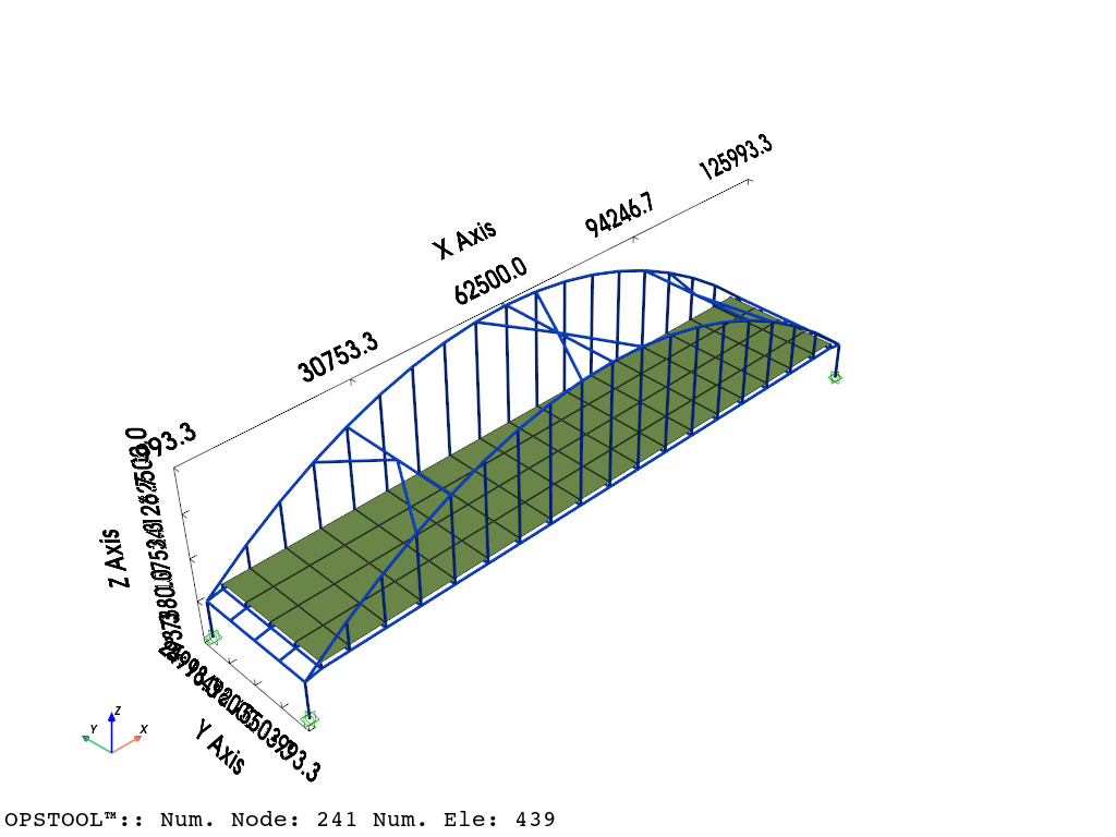
Here, we use a built-in example from opstool, which is an example of a deck arch bridge model primarily composed of frame elements and shell elements.

opst.load_ops_examples("ArchBridge2")
# or your model code here

We use the opstool.vis.pyvista.set_plot_props() function to predefine some common visualization properties, which will affect all subsequent visualizations of models, eigenvalues, and responses.

Model Geometry

opsvis.set_plot_props(point_size=0, line_width=3)

fig = opsvis.plot_model(show_outline=True)
fig.show()

Static Scene

Interactive Scene

Gravity Analysis

Apply the gravity load according to the mass in the model:

ops.timeSeries("Linear", 1)
ops.pattern("Plain", 1, 1)
_ = opst.pre.gen_grav_load(factor=-9810)

Analysis Parameters:

ops.system("BandGeneral")
# Create the constraint handler, the transformation method
ops.constraints("Transformation")
# Create the DOF numberer, the reverse Cuthill-McKee algorithm
ops.numberer("RCM")
# Create the convergence test, the norm of the residual with a tolerance of
# 1e-12 and a max number of iterations of 10
ops.test("NormDispIncr", 1.0e-12, 10, 3)
# Create the solution algorithm, a Newton-Raphson algorithm
ops.algorithm("Newton")
# Create the integration scheme, the LoadControl scheme using steps of 0.1
ops.integrator("LoadControl", 0.1)
# Create the analysis object
ops.analysis("Static")

Analysis and Saving Results

ODB = opst.post.CreateODB(odb_tag=1)
for i in range(10):
    ops.analyze(1)
    ODB.fetch_response_step()
ODB.save_response()

OPSTOOL™ ::  All responses data with _odb_tag = 1 saved in G:\opstool\docs\.opstool.output\RespStepData-1.odb!

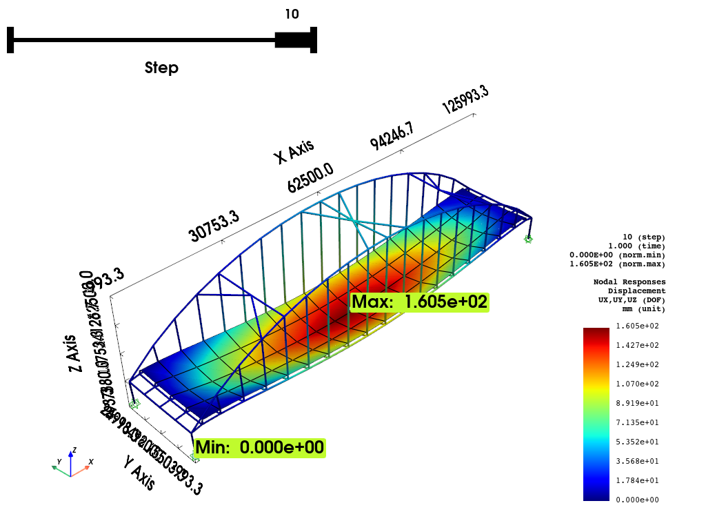
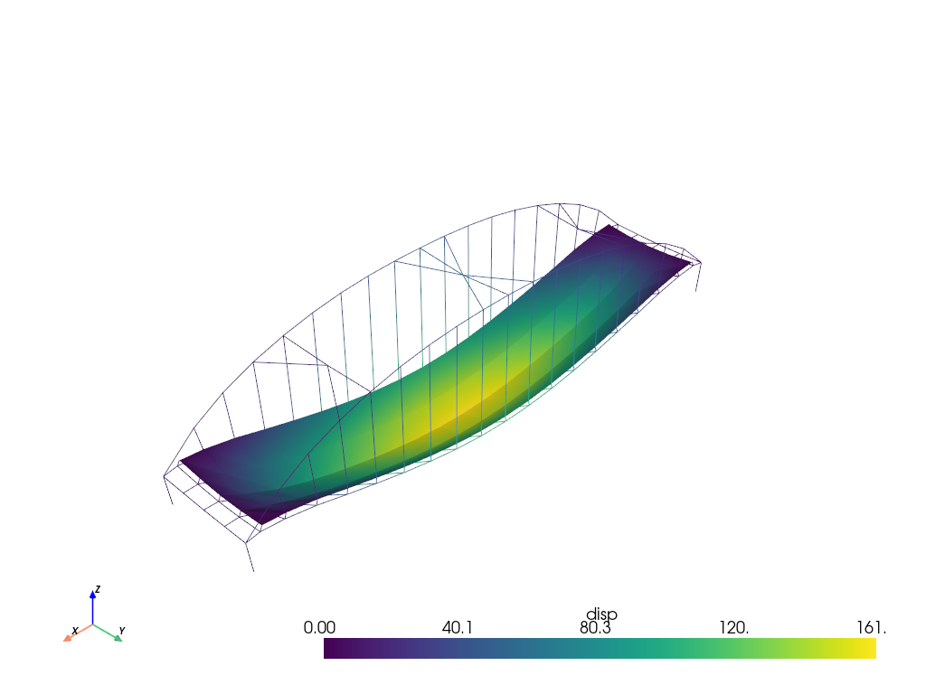
Nodal Responses Visualization

via Slides

opsvis.set_plot_props(scalar_bar_kargs={"title_font_size": 12, "label_font_size": 12})
fig = opsvis.plot_nodal_responses(
    odb_tag=1,
    slides=True,
    resp_type="disp",
    resp_dof=["UX", "UY", "UZ"],
    unit_symbol="mm",
    show_outline=True,
    defo_scale="auto",
)
fig.show()

Static Scene

Interactive Scene

OPSTOOL™ ::  Loading responses data from G:\opstool\docs\.opstool.output\RespStepData-1.odb ...

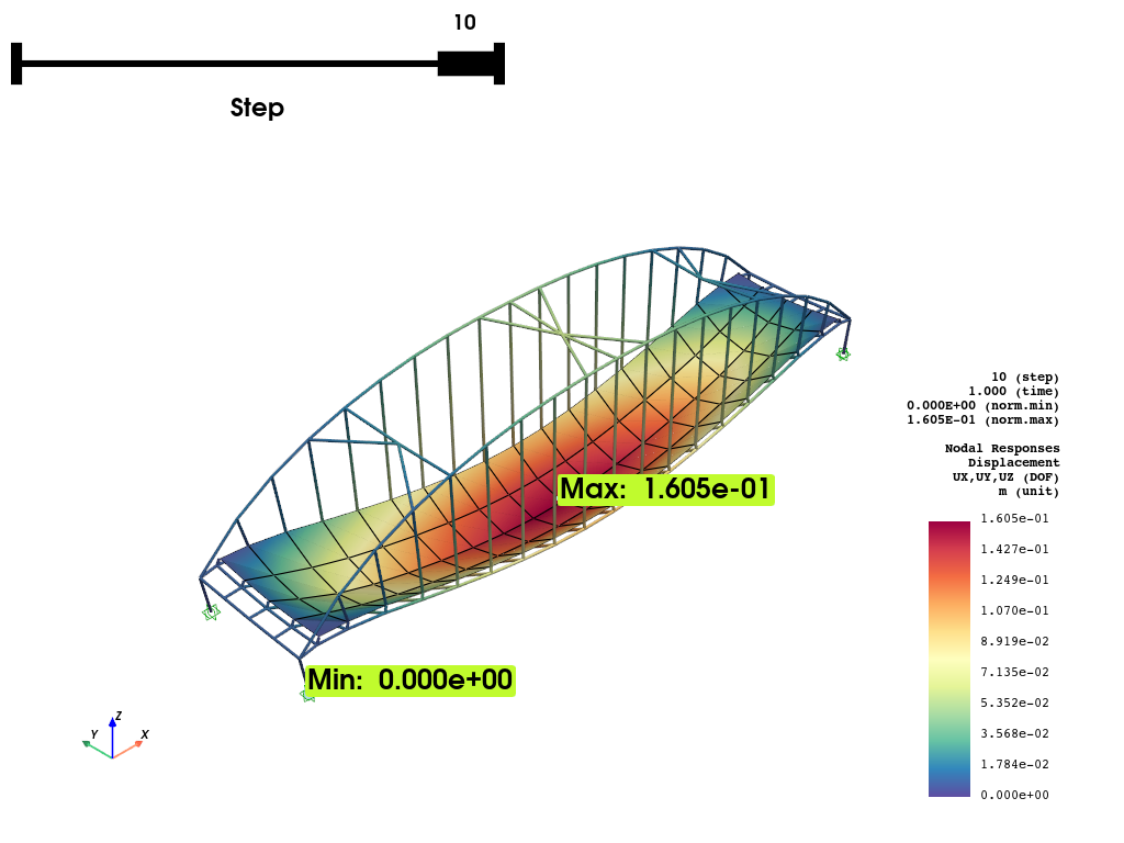
Change the unit dispaly

opsvis.set_plot_colors(cmap="Spectral_r")
fig = opsvis.plot_nodal_responses(
    odb_tag=1,
    slides=True,
    step=9,
    resp_type="disp",
    resp_dof=["UX", "UY", "UZ"],
    unit_symbol="m",
    unit_factor=1e-3,
    defo_scale=100,  # you can adjust the deformation scale factor here
)
fig.show()

Static Scene

Interactive Scene

OPSTOOL™ ::  Loading responses data from G:\opstool\docs\.opstool.output\RespStepData-1.odb ...

Animation

fig = opsvis.plot_nodal_responses_animation(
    odb_tag=1,
    framerate=2,
    defo_scale=100,
    savefig="images/NodalRespAnimation.gif",
    resp_type="disp",
    resp_dof=["UX", "UY", "UZ"],
    unit_symbol="m",
    unit_factor=1e-3,
)
fig.close()

OPSTOOL™ ::  Loading responses data from G:\opstool\docs\.opstool.output\RespStepData-1.odb ...
Animation has been saved to images/NodalRespAnimation.gif!

Interacting with Pyvista

Since version 1.0.18, opstool provides a function get_nodal_responses_dataset that returns a pyvista UnstructuredGrid so that you can take advantage of all the functionality on it.

grid = opsvis.get_nodal_responses_dataset(
    odb_tag=1,
    step="absMax",
    resp_type="disp",
    resp_dof=["UX", "UY", "UZ"],
    defo_scale=100,
)

OPSTOOL™ ::  Loading responses data from G:\opstool\docs\.opstool.output\RespStepData-1.odb ...

The name of the scalar data to be activated will be the passed in resp_type:

print(grid)
print(grid.active_scalars_name)

UnstructuredGrid (0x2a3988cdcc0)
  N Cells:    439
  N Points:   241
  X Bounds:   -8.820e+02, 1.259e+05
  Y Bounds:   -7.853e+01, 2.408e+04
  Z Bounds:   -8.045e+03, 2.775e+04
  N Arrays:   1
disp

You can call the plot method directly:

grid.plot()

Static Scene

Interactive Scene

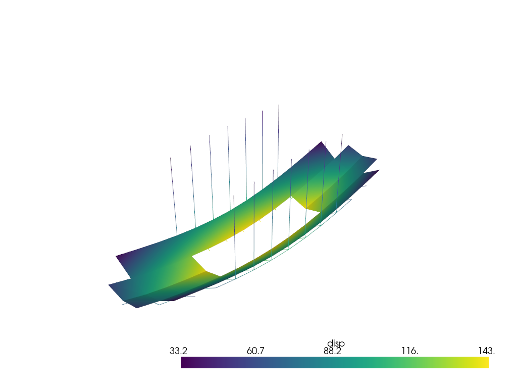
You can also use the filters provided by pyvista: DataSetFilters

For example, using some common filters: Using Common Filters

Apply a threshold over a data range

import pyvista as pv

threshed = grid.threshold([80, 120])

p = pv.Plotter()
p.add_mesh(threshed)
p.show()

Static Scene

Interactive Scene

More details can be found in the PyVista Examples.