Soil-Structure Interaction

This example originates from the GitHub repository maintained by Professor Quan Gu of Xiamen University. OpenSeesXMU

The TCL script has been translated into a Python script using opstool.pre.tcl2py For details, see: model.py

import matplotlib.pyplot as plt
import openseespy.opensees as ops
from utils.SSI_Gu_model import Model

import opstool as opst
import opstool.vis.pyvista as opsvis

Model()

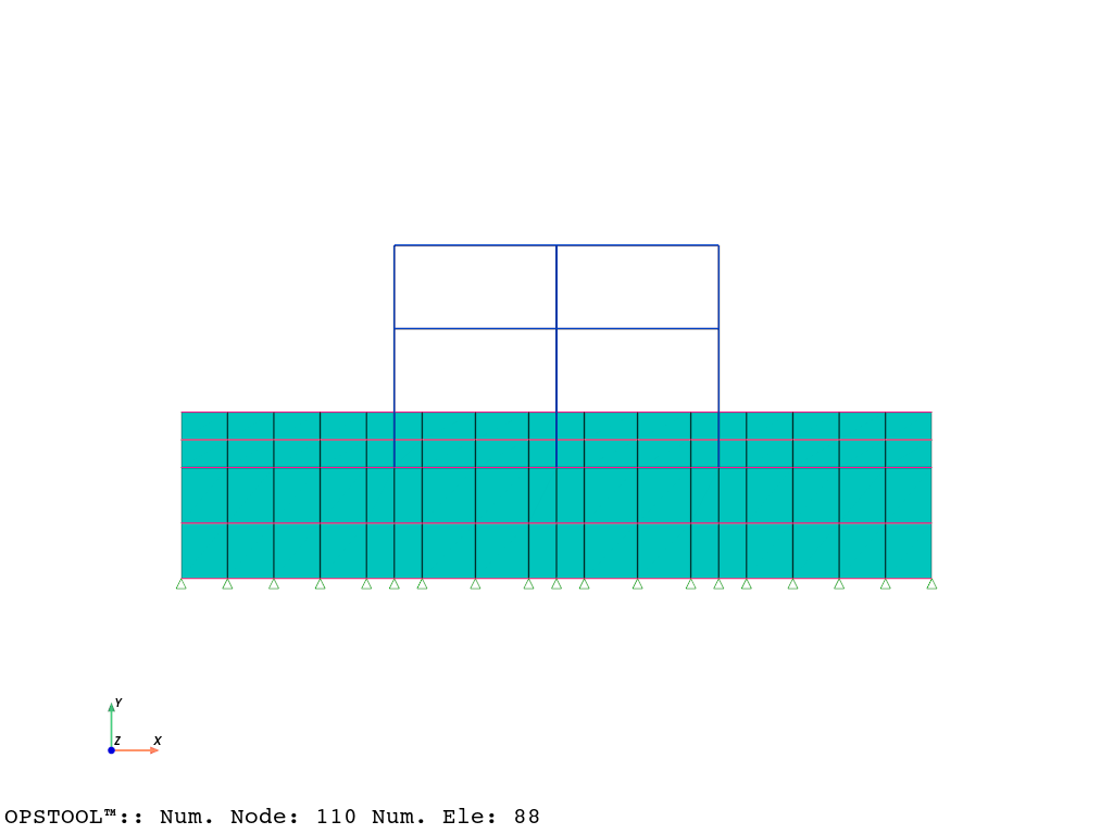
Visualize the model

fig = opsvis.plot_model()
fig.show()

Static Scene

Interactive Scene

Gravity analysis

ops.constraints("Transformation")
ops.numberer("RCM")
ops.test("NormDispIncr", 1e-06, 25, 2)
ops.integrator("LoadControl", 1, 1, 1, 1)
ops.algorithm("Newton")
ops.system("BandGeneral")
ops.analysis("Static")
ops.analyze(3)
print("soil gravity nonlinear analysis completed ...")

soil gravity nonlinear analysis completed ...

Earthquake analysis

ops.timeSeries("Path", 1, "-dt", 0.01, "-filePath", "utils/elcentro.txt", "-factor", 3)
ops.pattern("UniformExcitation", 1, 1, "-accel", 1)

ops.wipeAnalysis()
ops.constraints("Transformation")
ops.test("NormDispIncr", 1e-06, 25)
ops.algorithm("Newton")
ops.numberer("RCM")
ops.system("BandGeneral")
ops.integrator("Newmark", 0.55, 0.275625)
ops.analysis("Transient")

ODB = opst.post.CreateODB(
    odb_tag=1,
    save_every=500,  # save response every n steps
    compute_mechanical_measures=True,  # compute stress measures, strain measures, etc.
    project_gauss_to_nodes="copy",  # project gauss point responses to nodes, optional ["copy", "average", "extrapolate"]
)  # Create ODB object

for _ in range(2400):
    ops.analyze(1, 0.005)
    ODB.fetch_response_step()  # Fetch response for the current step
ODB.save_response()  # Save response

OPSTOOL™ ::  All responses data with _odb_tag = 1 saved in G:\opstool\docs\.opstool.output\RespStepData-1.odb!

Post-processing

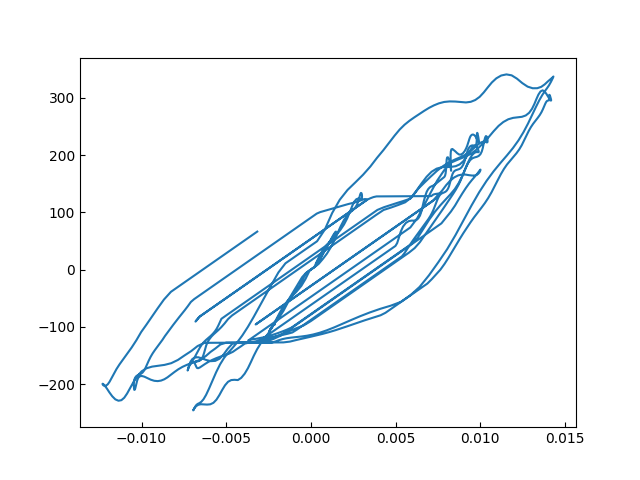
Frame Element Response

FrameResp = opst.post.get_element_responses(odb_tag=1, ele_type="Frame")

OPSTOOL™ ::  Loading Frame response data from G:\opstool\docs\.opstool.output\RespStepData-1.odb ...

f = FrameResp["sectionForces"].sel(eleTags=7, secDofs="MZ", secPoints=1)
d = FrameResp["sectionDeformations"].sel(eleTags=7, secDofs="MZ", secPoints=1)

plt.plot(d, f)
plt.show()

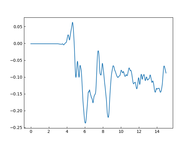
Nodal response

NodalResp = opst.post.get_nodal_responses(odb_tag=1)

OPSTOOL™ ::  Loading all response data from G:\opstool\docs\.opstool.output\RespStepData-1.odb ...

time = NodalResp.time
disp = NodalResp["disp"].sel(nodeTags=1, DOFs="UX")

plt.plot(time, disp)
plt.show()

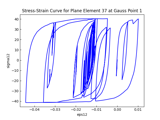
Plane Soil Element

PlaneResp = opst.post.get_element_responses(odb_tag=1, ele_type="Plane")
print(PlaneResp.coords)

OPSTOOL™ ::  Loading Plane response data from G:\opstool\docs\.opstool.output\RespStepData-1.odb ...
Coordinates:
  * time         (time) float32 10kB 0.0 3.005 3.01 3.015 ... 14.99 14.99 15.0
  * nodeTags     (nodeTags) int64 760B 16 17 36 35 18 37 ... 106 107 108 109 110
  * eleTags      (eleTags) int64 576B 17 18 19 20 21 22 23 ... 83 84 85 86 87 88
  * GaussPoints  (GaussPoints) int64 32B 1 2 3 4
  * strainDOFs   (strainDOFs) <U5 60B 'eps11' 'eps22' 'eps12'
  * stressDOFs   (stressDOFs) <U7 84B 'sigma11' 'sigma22' 'sigma12'
  * measures     (measures) <U9 288B 'p1' 'p2' 'p3' ... 'tau_oct' 'tau_max'

print(PlaneResp["Stresses"])

<xarray.DataArray 'Stresses' (time: 2401, eleTags: 72, GaussPoints: 4,
                              stressDOFs: 3)> Size: 8MB
array([[[[-7.87159348e+01, -9.81686630e+01, -3.99950528e+00],
         [-7.80784378e+01, -9.52057495e+01, -1.37933321e+01],
         [-1.49999466e+02, -1.43101654e+02, -1.27803211e+01],
         [-1.51964249e+02, -1.45000443e+02, -3.40683317e+00]],

        [[-8.32958908e+01, -9.66903687e+01, -1.96738453e+01],
         [-8.31516571e+01, -9.43495178e+01, -2.58833942e+01],
         [-1.65459122e+02, -1.54916794e+02, -2.47104702e+01],
         [-1.67807724e+02, -1.55793518e+02, -1.82695293e+01]],

        [[-9.39043198e+01, -1.04533356e+02, -2.98105240e+01],
         [-1.12065613e+02, -1.25788864e+02, -3.31040726e+01],
         [-2.01662155e+02, -1.97087021e+02, -3.35918312e+01],
         [-1.85142105e+02, -1.74861862e+02, -3.02270164e+01]],

        ...,

        [[-2.57066860e+01, -1.26524124e+01, -2.88750362e+00],
         [-2.89141922e+01, -1.80301628e+01,  4.06571627e+00],
         [-8.58915234e+00, -5.75890732e+00,  3.80573177e+00],
...
         [-4.00514618e+02, -4.02227692e+02, -2.83885479e+01],
         [-3.16135529e+02, -3.12804596e+02, -2.82437687e+01]],

        ...,

        [[ 8.08007812e+01,  4.38142891e+01,  2.07107735e+00],
         [ 7.48245926e+01,  4.77452888e+01,  4.19595814e+00],
         [-9.49740982e+01, -1.19399628e+02,  9.50423336e+00],
         [-8.74431534e+01, -1.23985062e+02,  6.59181833e+00]],

        [[ 3.59630966e+01,  3.63306885e+01,  7.11050081e+00],
         [-5.46431274e+01, -4.51247559e+01,  1.37734306e+00],
         [-7.89630966e+01, -6.29889412e+01, -1.60193717e+00],
         [ 1.22680483e+01,  1.81050110e+01,  5.86197567e+00]],

        [[-2.66656780e+01, -6.56829655e-01,  1.67323387e+00],
         [-6.33080597e+01, -3.74379807e+01,  1.33412695e+00],
         [-2.97291107e+01,  1.95029926e+00, -3.60264039e+00],
         [ 8.35825825e+00,  3.75435410e+01, -1.00076556e+00]]]],
      shape=(2401, 72, 4, 3), dtype=float32)
Coordinates:
  * time         (time) float32 10kB 0.0 3.005 3.01 3.015 ... 14.99 14.99 15.0
  * eleTags      (eleTags) int64 576B 17 18 19 20 21 22 23 ... 83 84 85 86 87 88
  * GaussPoints  (GaussPoints) int64 32B 1 2 3 4
  * stressDOFs   (stressDOFs) <U7 84B 'sigma11' 'sigma22' 'sigma12'

s = PlaneResp["Stresses"].sel(eleTags=37, GaussPoints=1, stressDOFs="sigma12")
e = PlaneResp["Strains"].sel(eleTags=37, GaussPoints=1, strainDOFs="eps12")

plt.plot(e, s, c="blue")
plt.xlabel("eps12")
plt.ylabel("sigma12")
plt.title("Stress-Strain Curve for Plane Element 37 at Gauss Point 1")
plt.show()

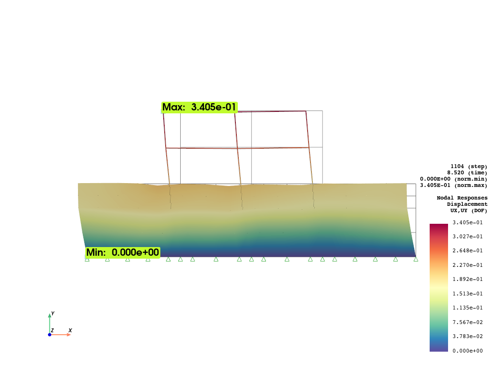
Plotting the nodal responses with deformed shape

opsvis.set_plot_props(
    cmap="Spectral_r",
    point_size=0.0,
    scalar_bar_kargs={"title_font_size": 12, "label_font_size": 12, "position_x": 0.865},
    show_mesh_edges=False,
)

fig = opst.vis.pyvista.plot_nodal_responses(
    odb_tag=1,
    slides=False,
    step="absMax",
    resp_type="disp",
    resp_dof=("UX", "UY"),
    show_defo=True,
    defo_scale=5,
    show_undeformed=True,
)
fig.show()

Static Scene

Interactive Scene

OPSTOOL™ ::  Loading responses data from G:\opstool\docs\.opstool.output\RespStepData-1.odb ...

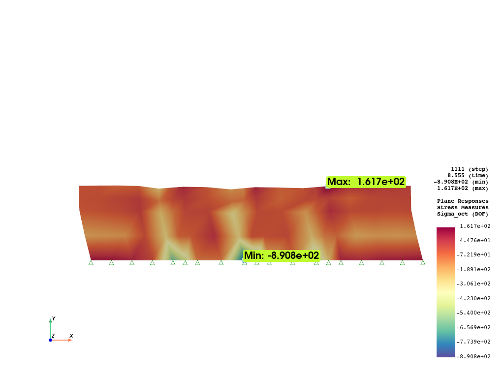
Plotting the plane element stresses

fig = opst.vis.pyvista.plot_unstruct_responses(
    odb_tag=1,
    slides=False,
    step="absMax",
    ele_type="Plane",
    resp_type="StressesAtNodes",
    resp_dof="sigma_oct",  # hydrostatic pressure
    show_defo=True,
    defo_scale="auto",
    show_model=True,
)
fig.show()

Static Scene

Interactive Scene

OPSTOOL™ ::  Loading responses data from G:\opstool\docs\.opstool.output\RespStepData-1.odb ...

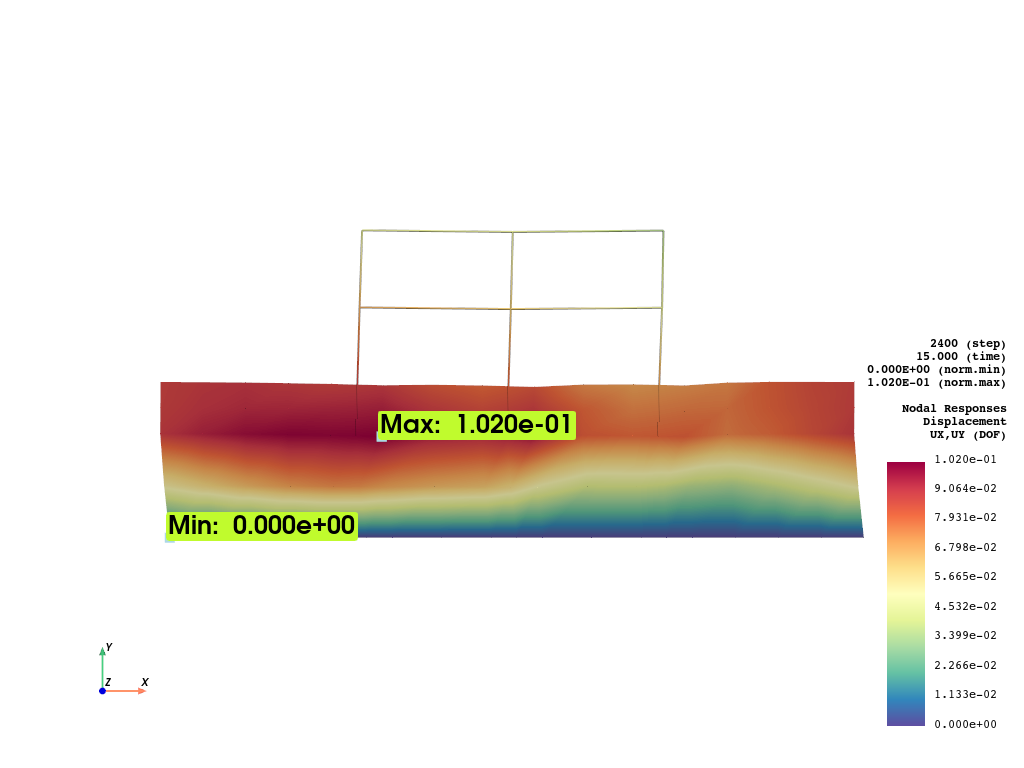
Plotting the deformation animation

fig = opst.vis.pyvista.plot_nodal_responses_animation(
    odb_tag=1,
    framerate=50,  # Frames per second
    resp_type="disp",
    resp_dof=("UX", "UY"),
    show_defo=True,
    defo_scale=5,
    savefig="images/nodal_disp_animation_ssi.mp4",
)
fig.show()

Static Scene

Interactive Scene

OPSTOOL™ ::  Loading responses data from G:\opstool\docs\.opstool.output\RespStepData-1.odb ...
Animation has been saved to images/nodal_disp_animation_ssi.mp4!

Clean up

fig.close()

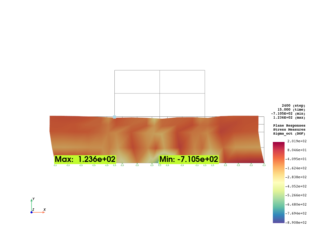
fig = opst.vis.pyvista.plot_unstruct_responses_animation(
    odb_tag=1,
    framerate=50,  # Frames per second
    ele_type="Plane",
    resp_type="StressesAtNodes",
    resp_dof="sigma_oct",
    show_defo=True,
    defo_scale=10,
    show_model=True,
    savefig="images/stress_animation_ssi.mp4",
)
fig.show()

Static Scene

Interactive Scene

OPSTOOL™ ::  Loading responses data from G:\opstool\docs\.opstool.output\RespStepData-1.odb ...
Animation has been saved as images/stress_animation_ssi.mp4!

Clean up

fig.close()