Shell Element Responses

import openseespy.opensees as ops

import opstool as opst
import opstool.vis.pyvista as opsvis

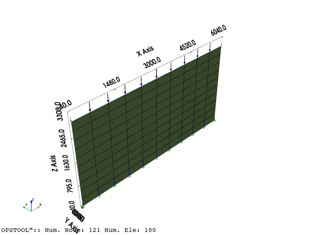
Model and gravity load

opst.load_ops_examples("Shell3D")

ops.timeSeries("Linear", 1)
ops.pattern("Plain", 1, 1)
_ = opst.pre.gen_grav_load(direction="Z", factor=-9810)

The original Tcl file comes from http://www.dinochen.com/, and the Python version is converted by opstool.tcl2py().

opsvis.set_plot_props(point_size=0, line_width=3)  # notebook=False for practical use
fig = opsvis.plot_model(show_nodal_loads=True, show_ele_loads=True, show_outline=True)
fig.show()

Static Scene

Interactive Scene

Gravity analysis

ops.constraints("Transformation")
ops.numberer("RCM")
ops.system("BandGeneral")
ops.test("NormDispIncr", 1.0e-8, 6, 2)
ops.algorithm("Linear")
ops.integrator("LoadControl", 0.1)
ops.analysis("Static")

Save the responses

ODB = opst.post.CreateODB(
    odb_tag=1,
    project_gauss_to_nodes="copy",  # project gauss point responses to nodes, optional ["copy", "average", "extrapolate"]
)
for _ in range(10):
    ops.analyze(1)
    ODB.fetch_response_step()
ODB.save_response()

OPSTOOL™ ::  All responses data with _odb_tag = 1 saved in G:\opstool\docs\.opstool.output\RespStepData-1.odb!

Visualize the results

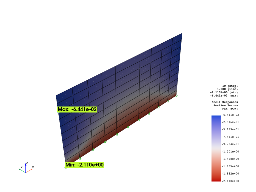
Nodal responses, project_gauss_to_nodes needs to be set to “copy”, “average”, or “extrapolate” when creating the ODB

opsvis.set_plot_props(cmap="coolwarm_r", show_mesh_edges=True)

fig = opsvis.plot_unstruct_responses(
    odb_tag=1,
    slides=False,
    step="absMax",
    ele_type="Shell",
    resp_type="sectionForcesAtNodes",  # nodal response, "AtNodes"
    resp_dof="FXX",
)
fig.show()

Static Scene

Interactive Scene

OPSTOOL™ ::  Loading responses data from G:\opstool\docs\.opstool.output\RespStepData-1.odb ...

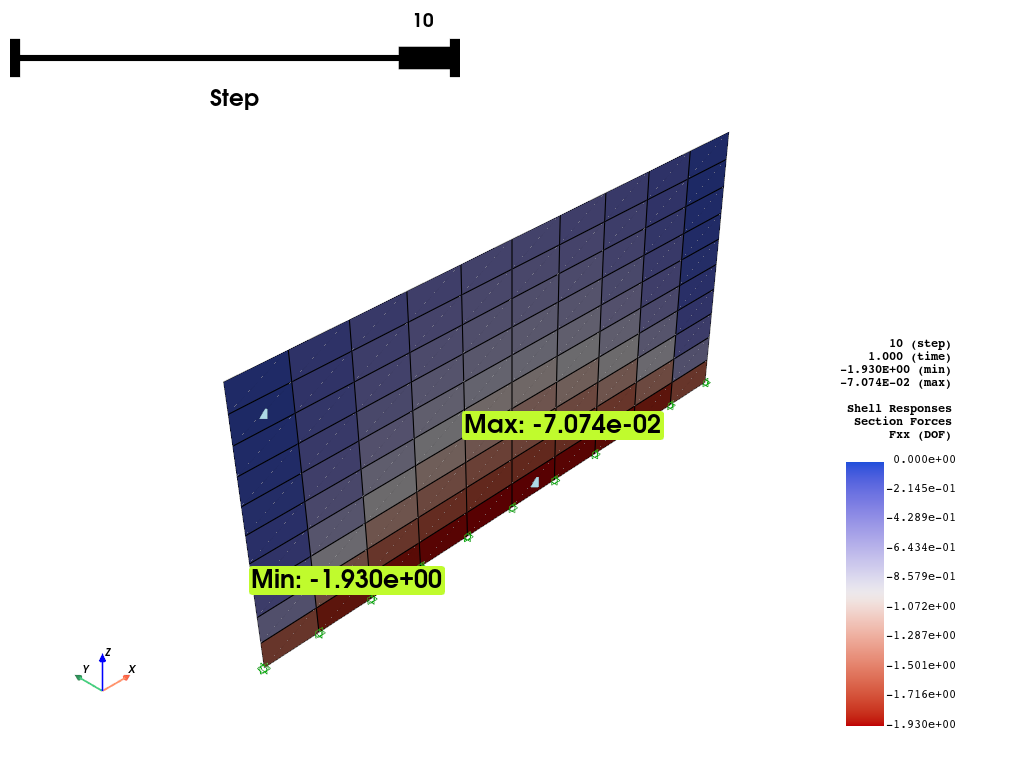
Display the responses at each element, all gauss points will be averaged to the element level.

fig = opsvis.plot_unstruct_responses(
    odb_tag=1,
    slides=True,
    ele_type="Shell",
    resp_type="sectionForces",  # element response, "AtGaussPoints", will be averaged to each element
    resp_dof="FXX",
)
fig.show()

Static Scene

Interactive Scene

OPSTOOL™ ::  Loading responses data from G:\opstool\docs\.opstool.output\RespStepData-1.odb ...

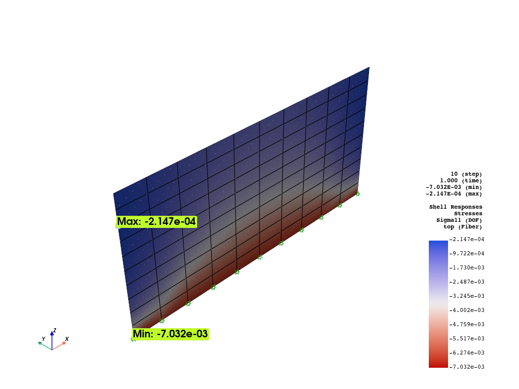
Fiber point stress can be plotted as well, but it requires a shell_fiber_loc to be assigned. sphinx_gallery_thumbnail_number = 5

fig = opsvis.plot_unstruct_responses(
    odb_tag=1,
    slides=False,
    step="absMax",
    ele_type="Shell",
    resp_type="StressesAtNodes",  # nodal stress response, "AtNodes"
    resp_dof="sigma11",  # sigma11, sigma22, sigma12, sigma13, sigma23
    shell_fiber_loc="top",  # shell_fiber_loc can be "top", "bottom", or "mid" for shell elements, also int
)
fig.show()

Static Scene

Interactive Scene

OPSTOOL™ ::  Loading responses data from G:\opstool\docs\.opstool.output\RespStepData-1.odb ...

Interacting with Pyvista

Since version 1.0.18, opstool provides a function get_unstruct_responses_dataset that returns a pyvista UnstructuredGrid so that you can take advantage of all the functionality on it.

import pyvista as pv

grid = opsvis.get_unstruct_responses_dataset(
    odb_tag=1,
    step="absMax",
    ele_type="Shell",
    resp_type="StressesAtNodes",  # nodal stress response, "AtNodes"
    resp_dof="sigma11",  # sigma11, sigma22, sigma12, sigma13, sigma23
    shell_fiber_loc="top",  # shell_fiber_loc can be "top", "bottom", or "mid" for shell elements, also int
)

OPSTOOL™ ::  Loading responses data from G:\opstool\docs\.opstool.output\RespStepData-1.odb ...

print(grid)
print("--" * 20)
print(grid.active_scalars_name)

UnstructuredGrid (0x2a3918e6620)
  N Cells:    100
  N Points:   121
  X Bounds:   0.000e+00, 6.000e+03
  Y Bounds:   0.000e+00, 0.000e+00
  Z Bounds:   0.000e+00, 3.000e+03
  N Arrays:   1
----------------------------------------
StressesAtNodes

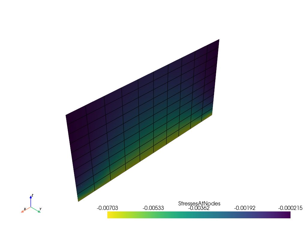
grid.plot(show_edges=True, cmap="viridis_r", show_scalar_bar=True)

Static Scene

Interactive Scene

Plot Over Line

print(grid.bounds)

BoundsTuple(x_min =    0.0,
            x_max = 6000.0,
            y_min =    0.0,
            y_max =    0.0,
            z_min =    0.0,
            z_max = 3000.0)

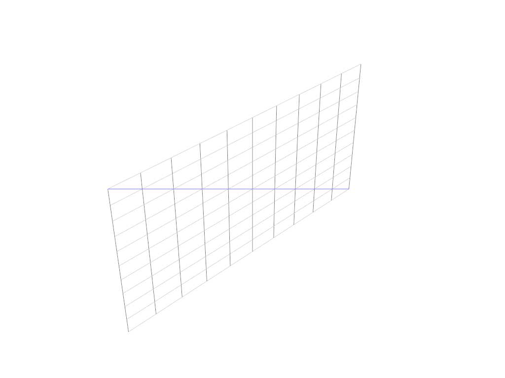
a = [0, 0, 0]
b = [6000, 0, 3000]  # A line from (0, 0, 0) to (0, 0, 1)

# Preview how this line intersects this mesh
line = pv.Line(a, b)

p = pv.Plotter()
p.add_mesh(grid, style="wireframe", color="w")
p.add_mesh(line, color="b")
p.show()

Static Scene

Interactive Scene

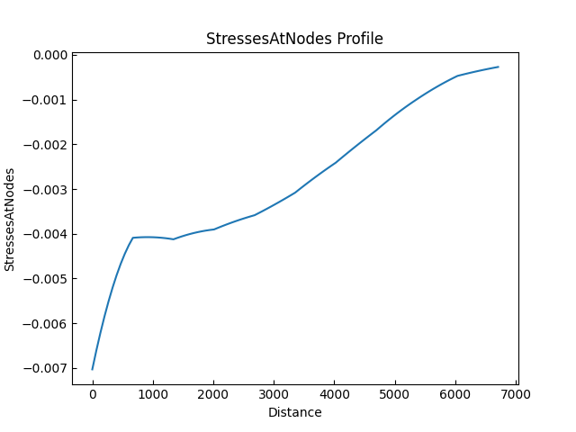
grid.plot_over_line(a, b)

More details can be found in the PyVista Examples.