Note
Go to the end to download the full example code.
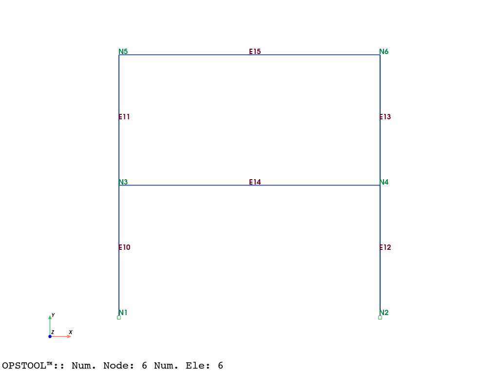
Two storey steel moment frame with W-sections for displacement-controlled sensitivity analysis
This document will teach you how to use opstool to post-process sensitivity analysis.
The source code is developed by Marin Grubišić at University of Osijek, Croatia. The numerical model with the associated analysis was described in detail by Prof. Michael Scott in the Portwood Digital blog.
import matplotlib.pyplot as plt
import openseespy.opensees as ops

import opstool as opst
OpenSees Model
Use the unit system provided by opstool:
length_unit = "inch"
force_unit = "kip"
UNIT = opst.pre.UnitSystem(length=length_unit, force=force_unit, time="sec")
Define model
# Create ModelBuilder
# -------------------
ops.wipe()
ops.model("basic", "-ndm", 2, "-ndf", 3)

# Create nodes
# ------------
ops.node(1, 0.0, 0.0)  # Ground Level
ops.node(2, 30 * UNIT.ft, 0.0)
ops.node(3, 0.0, 15 * UNIT.ft)  # 1st Floor Level
ops.node(4, 30 * UNIT.ft, 15 * UNIT.ft)
ops.node(5, 0.0, 2 * 15 * UNIT.ft)  # 2nd Floor Level
ops.node(6, 30 * UNIT.ft, 2 * 15 * UNIT.ft)

# Fix supports at base of columns
# -------------------------------
ops.fix(1, 1, 1, 1)
ops.fix(2, 1, 1, 1)

# Define material
# ---------------
matTag = 1
Fy = 50.0 * UNIT.ksi  # Yield stress
Es = 29000.0 * UNIT.ksi  # Modulus of Elasticity of Steel
b = 1 / 100  # 1% Strain hardening ratio

# Sensitivity-ready steel materials: Hardening, Steel01, SteelMP, BoucWen, SteelBRB, StainlessECThermal, SteelECThermal, ...
ops.uniaxialMaterial("Steel01", matTag, Fy, Es, b)
# ops.uniaxialMaterial("SteelMP", matTag, Fy, Es, b)

# Define sections
# ---------------
# Sections defined with "canned" section ("WFSection2d"), otherwise use a FiberSection object (ops.section("Fiber",...))
colSecTag, beamSecTag = 1, 2
WSection = {
    "W18x76": [
        18.2 * UNIT.inch,
        0.425 * UNIT.inch,
        11.04 * UNIT.inch,
        0.68 * UNIT.inch,
    ],  # [d, tw, bf, tf]
    "W14X90": [
        14.02 * UNIT.inch,
        0.44 * UNIT.inch,
        14.52 * UNIT.inch,
        0.71 * UNIT.inch,
    ],  # [d, tw, bf, tf]
}

#                          secTag,    matTag, [d, tw, bf, tf],    Nfw, Nff
ops.section("WFSection2d", colSecTag, matTag, *WSection["W14X90"], 20, 4)  # Column section
ops.section("WFSection2d", beamSecTag, matTag, *WSection["W18x76"], 20, 4)  # Beam section

# Define elements
# ---------------
colTransTag, beamTransTag = 1, 2
# Linear, PDelta, Corotational
ops.geomTransf("Corotational", colTransTag)
ops.geomTransf("Linear", beamTransTag)

colIntTag, beamIntTag = 1, 2
nip = 5
# Lobatto, Legendre, NewtonCotes, Radau, Trapezoidal, CompositeSimpson
(ops.beamIntegration("Lobatto", colIntTag, colSecTag, nip),)
ops.beamIntegration("Lobatto", beamIntTag, beamSecTag, nip)

# Column elements
ops.element("forceBeamColumn", 10, 1, 3, colTransTag, colIntTag, "-mass", 0.0)
ops.element("forceBeamColumn", 11, 3, 5, colTransTag, colIntTag, "-mass", 0.0)
ops.element("forceBeamColumn", 12, 2, 4, colTransTag, colIntTag, "-mass", 0.0)
ops.element("forceBeamColumn", 13, 4, 6, colTransTag, colIntTag, "-mass", 0.0)

# Beam elements
ops.element("forceBeamColumn", 14, 3, 4, beamTransTag, beamIntTag, "-mass", 0.0)
ops.element("forceBeamColumn", 15, 5, 6, beamTransTag, beamIntTag, "-mass", 0.0)

# Create a Plain load pattern with a Linear TimeSeries
# ----------------------------------------------------
ops.timeSeries("Linear", 1)
ops.pattern("Plain", 1, 1)
Define Sensitivity Parameters
Each parameter must be unique in the FE domain, and all parameter tags MUST be numbered sequentially starting from 1!
ops.parameter(1)  # Blank parameters
ops.parameter(2)
ops.parameter(3)
for ele in [10, 11, 12, 13]:  # Only column elements
    ops.addToParameter(1, "element", ele, "E")  # "E"
    # Check the sensitivity parameter name in *.cpp files ("sigmaY" or "fy", somewhere also "Fy")
    # https://github.com/OpenSees/OpenSees/blob/master/SRC/material/uniaxial/Steel02.cpp
    ops.addToParameter(2, "element", ele, "fy")  # "sigmaY" or "fy" or "Fy"
    ops.addToParameter(3, "element", ele, "b")  # "b"

ParamSym = {1: "E", 2: "F_y", 3: "b"}
ParamVars = {1: Es, 2: Fy, 3: b}
Visualize the model
opst.vis.pyvista.plot_model(show_node_numbering=True, show_ele_numbering=True).show()
Run gravity analysis (in 10 steps)
steps = 10

ops.wipeAnalysis()
ops.system("BandGeneral")
ops.numberer("RCM")
ops.constraints("Transformation")
ops.test("NormDispIncr", 1.0e-12, 10, 3)
ops.algorithm("Newton")  # KrylovNewton
ops.integrator("LoadControl", 1 / steps)
ops.analysis("Static")
ops.analyze(steps)
# Set the gravity loads to be constant & reset the time in the domain
ops.loadConst("-time", 0.0)
ops.wipeAnalysis()
Run sensitivity and pushover analysis
# Define nodal loads for pushover analysis
ops.pattern("Plain", 2, 1)  # new load pattern 2
# Create nodal loads at nodes 3 & 5
#       nd  FX   FY   MZ
ops.load(3, 1 / 3, 0.0, 0.0)
ops.load(5, 2 / 3, 0.0, 0.0)
P = 1 / 3 + 2 / 3  # Total load
Control node and dof for pushover analysis
ctrlNode = 5
dof = 1
Dincr = (1 / 25) * UNIT.inch
max_disp = 20 * UNIT.inch
Setting up the analysis algorithm
ops.wipeAnalysis()
ops.system("BandGeneral")
ops.constraints("Transformation")
ops.numberer("RCM")
ops.test("NormDispIncr", 1.0e-8, 10)
ops.algorithm("Newton")
# Change the integration scheme to be displacement control
#                                     node      dof  init Jd min max
ops.integrator("DisplacementControl", ctrlNode, dof, Dincr)
ops.analysis("Static")
ops.sensitivityAlgorithm("-computeAtEachStep")  # automatically compute sensitivity at the end of each step
Run the analysis
Here we use the [smart analysis algorithm](https://opstool.readthedocs.io/en/latest/src/api/_autosummary/opstool.anlys.SmartAnalyze.html#opstool.anlys.SmartAnalyze) provided by opstool, which can help convergence.
It should be noted that since the integrator may be reset internally, you need to call the set_sensitivity_algorithm method to inform you that you are running sensitivity analysis so that the sensitivity analysis algorithm is reset every time the integrator is reset.
analysis = opst.anlys.SmartAnalyze(
    analysis_type="Static",
    tryAlterAlgoTypes=True,
    algoTypes=[40, 10],
    printPer=100,
)
analysis.set_sensitivity_algorithm("-computeAtEachStep")
segs = analysis.static_split([max_disp], Dincr)
ODB = opst.post.CreateODB("sensitivity-pushover", save_sensitivity_resp=True)
for seg in segs:
    analysis.StaticAnalyze(node=ctrlNode, dof=dof, seg=seg)
    # ops.analyze(1)
    ODB.fetch_response_step()
ODB.save_response()
🚀 OPSTOOL::SmartAnalyze:   0%|                                                    | 0/500 [00:00<?, ? step/s]
🚀 OPSTOOL::SmartAnalyze:   8%|███▌                                      | 42/500 [00:00<00:01, 419.03 step/s]
🚀 OPSTOOL::SmartAnalyze:  33%|█████████████▋                           | 167/500 [00:00<00:00, 905.52 step/s]
🚀 OPSTOOL::SmartAnalyze:  58%|███████████████████████                 | 289/500 [00:00<00:00, 1047.61 step/s]
🚀 OPSTOOL::SmartAnalyze:  82%|████████████████████████████████▉       | 412/500 [00:00<00:00, 1118.53 step/s]
🚀 OPSTOOL::SmartAnalyze: 100%|████████████████████████████████████████| 500/500 [00:00<00:00, 1118.53 step/s]
🚀 OPSTOOL::SmartAnalyze: 100%|████████████████████████████████████████| 500/500 [00:00<00:00, 1052.70 step/s]
Note: OpenSees LogFile has been generated in .SmartAnalyze-OpenSees.log.
>>> 🎉 OPSTOOL::SmartAnalyze:: Successfully finished! Time consumption: 0.475 s. 🎉
OPSTOOL™ ::  All responses data with _odb_tag = sensitivity-pushover saved in
G:\opstool\docs\.opstool.output\RespStepData-sensitivity-pushover.odb!
Post-processing
ctrlNode = 5  # Node 5
dof = "UX"  # 1st DOF (X direction)
Loading node response
node_resp = opst.post.get_nodal_responses(odb_tag="sensitivity-pushover")
print("data variables:", node_resp.data_vars)
print("-" * 100)
print("dimensions:", node_resp.dims)
print("-" * 100)
print("coordinates:", node_resp.coords)
OPSTOOL™ ::  Loading all response data from
G:\opstool\docs\.opstool.output\RespStepData-sensitivity-pushover.odb ...
data variables: Data variables:
    accel               (time, nodeTags, DOFs) float32 72kB 0.0 0.0 ... 0.0 0.0
    disp                (time, nodeTags, DOFs) float32 72kB 0.0 0.0 ... -0.02203
    pressure            (time, nodeTags) float32 12kB 0.0 0.0 0.0 ... 0.0 0.0
    rayleighForces      (time, nodeTags, DOFs) float32 72kB 0.0 0.0 ... 0.0 0.0
    reaction            (time, nodeTags, DOFs) float32 72kB 0.0 ... -1.819e-11
    reactionIncInertia  (time, nodeTags, DOFs) float32 72kB 0.0 ... -1.819e-11
    vel                 (time, nodeTags, DOFs) float32 72kB 0.0 0.0 ... 0.0 0.0
----------------------------------------------------------------------------------------------------
dimensions: FrozenMappingWarningOnValuesAccess({'time': 501, 'nodeTags': 6, 'DOFs': 6})
----------------------------------------------------------------------------------------------------
coordinates: Coordinates:
  * time      (time) float32 2kB 0.0 1.138 2.277 3.415 ... 175.9 176.0 176.0
  * nodeTags  (nodeTags) int64 48B 1 2 3 4 5 6
  * DOFs      (DOFs) <U2 48B 'UX' 'UY' 'UZ' 'RX' 'RY' 'RZ'
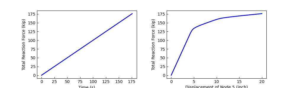
We use the .sel method to retrieve the displacement of node 5 on UX and total reaction force:
times = node_resp["time"].data
disp = node_resp["disp"].sel(nodeTags=ctrlNode, DOFs=dof)
force = -node_resp["reaction"].sel(DOFs=dof).sum(dim="nodeTags")
Plotting
fig, axs = plt.subplots(1, 2, figsize=(10, 3))
axs[0].plot(times, force, lw=2, color="blue")
axs[0].set_xlabel("Time (s)")
axs[1].plot(disp, force, lw=2, color="blue")
axs[1].set_xlabel(f"Displacement of Node {ctrlNode} ({length_unit})")
for ax in axs:
    ax.set_ylabel(f"Total Reaction Force ({force_unit})")
    # ax.grid()
plt.subplots_adjust(wspace=0.3)
plt.show()
Loading the sensitivity response data
sens_resp = opst.post.get_sensitivity_responses(odb_tag="sensitivity-pushover")
print("data variables:", sens_resp.data_vars)
print("-" * 100)
print("dimensions:", sens_resp.dims)
print("-" * 100)
print("coordinates:", sens_resp.coords)
OPSTOOL™ ::  Loading response data from G:\opstool\docs\.opstool.output\RespStepData-sensitivity-pushover.odb
...
data variables: Data variables:
    accel     (time, paraTags, nodeTags, DOFs) float32 216kB 0.0 0.0 ... 0.0 0.0
    disp      (time, paraTags, nodeTags, DOFs) float32 216kB 0.0 0.0 ... 0.4655
    lambdas   (time, paraTags, patternTags) float32 12kB 0.0 0.0 ... 1.111e+03
    pressure  (time, paraTags, nodeTags) float32 36kB 0.0 0.0 0.0 ... 0.0 0.0
    vel       (time, paraTags, nodeTags, DOFs) float32 216kB 0.0 0.0 ... 0.0 0.0
----------------------------------------------------------------------------------------------------
dimensions: FrozenMappingWarningOnValuesAccess({'time': 501, 'paraTags': 3, 'nodeTags': 6, 'DOFs': 6, 'patternTags': 2})
----------------------------------------------------------------------------------------------------
coordinates: Coordinates:
  * paraTags     (paraTags) int64 24B 1 2 3
  * nodeTags     (nodeTags) int64 48B 1 2 3 4 5 6
  * DOFs         (DOFs) <U2 48B 'UX' 'UY' 'UZ' 'RX' 'RY' 'RZ'
  * patternTags  (patternTags) int64 16B 1 2
Get all parameter tags:
paraTags = sens_resp.paraTags.data
print("parameter tags:", paraTags)
parameter tags: [1 2 3]
Sensitivity of load multipliers to various parameters
Retrieve the sensitivity of the load multiplier to various parameters in load pattern 2:
sens_lambda = sens_resp["lambdas"].sel(patternTags=2)
print(sens_lambda)
<xarray.DataArray 'lambdas' (time: 501, paraTags: 3)> Size: 6kB
array([[0.0000000e+00, 0.0000000e+00, 0.0000000e+00],
       [1.9715560e-05, 0.0000000e+00, 3.6402207e-02],
       [3.9431176e-05, 0.0000000e+00, 7.2804511e-02],
       ...,
       [5.0192908e-04, 1.4227666e+00, 1.1059608e+03],
       [5.0287606e-04, 1.4227755e+00, 1.1085642e+03],
       [5.0382304e-04, 1.4227844e+00, 1.1111677e+03]],
      shape=(501, 3), dtype=float32)
Coordinates:
  * paraTags     (paraTags) int64 24B 1 2 3
    patternTags  int64 8B 2
Dimensions without coordinates: time
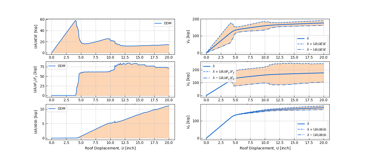
Plotting
The left column shows the sensitivity of load multiplier \(\lambda\) to each parameter \(P\) and the product of the parameter value:
The right column shows the hysteresis diagram of displacement \(U\) and total reaction force \(V_b\), where the \(\lambda\) includes a sensitivity change of 1 times, i.e., \(\left( \partial \lambda/\partial {P} \right){P}\)
fig, axs = plt.subplots(len(paraTags), 2, figsize=(7 * 2, 2 * len(paraTags)))

for j, para_tag in enumerate(paraTags):
    para_value = ParamVars[para_tag]
    para_sym = ParamSym[para_tag]
    sens = sens_lambda.sel(paraTags=para_tag)
    # Subplot #i
    # ----------
    axs[j, 0].plot(disp, sens * para_value, c="#136ad5", linewidth=1.5, label="DDM")
    axs[j, 0].fill_between(disp, sens * para_value, 0.0, color="#fb8a2e", alpha=0.35)
    axs[j, 0].set_ylabel(f"$(\\partial \\lambda/\\partial {para_sym}){para_sym}$ [{force_unit}]")
    axs[j, 0].legend(fontsize=9)

    # Subplot #ii
    # -----------
    axs[j, 1].plot(disp, force, c="#136ad5", linewidth=2.0, label="$\\lambda$")
    axs[j, 1].plot(
        disp,
        force + sens * para_value,
        c="#136ad5",
        ls="--",
        linewidth=1.5,
        label=f"$\\lambda + (\\partial \\lambda/\\partial {para_sym}){para_sym}$",
    )
    axs[j, 1].plot(
        disp,
        force - sens * para_value,
        c="#136ad5",
        ls="-.",
        linewidth=1.5,
        label=f"$\\lambda - (\\partial \\lambda/\\partial {para_sym}){para_sym}$",
    )
    axs[j, 1].fill_between(
        disp,
        force + sens * para_value,
        force - sens * para_value,
        color="#fb8a2e",
        alpha=0.35,
    )

    axs[j, 1].set_ylabel(f"$V_b$ [{force_unit}]")
    axs[j, 1].legend(fontsize=9)

for ax in axs.flat:
    ax.tick_params(direction="in", length=5, colors="k", width=0.75)
    ax.grid(True, color="silver", linestyle="solid", linewidth=0.75, alpha=0.75)
    if j == 2:
        ax.set_xlabel(f"Roof Displacement, $U$ [{length_unit}]")
plt.subplots_adjust(wspace=0.2)
plt.show()
Total running time of the script: (0 minutes 2.035 seconds)