Gmsh2OPS: Case 2

This example demonstrates how to read a GMSH model by physical groups and convert it to an OpenSeesPy model using the Gmsh2OPS class from the opstool library.

Gmsh model

This example is based on GMSH Example t15.

import gmsh

gmsh.initialize()

# Copied from `t1.py'...
lc = 1e-2
gmsh.model.geo.addPoint(0, 0, 0, lc, 1)
gmsh.model.geo.addPoint(0.1, 0, 0, lc, 2)
gmsh.model.geo.addPoint(0.1, 0.3, 0, lc, 3)
gmsh.model.geo.addPoint(0, 0.3, 0, lc, 4)
gmsh.model.geo.addLine(1, 2, 1)
gmsh.model.geo.addLine(3, 2, 2)
gmsh.model.geo.addLine(3, 4, 3)
gmsh.model.geo.addLine(4, 1, 4)
gmsh.model.geo.addCurveLoop([4, 1, -2, 3], 1)
gmsh.model.geo.addPlaneSurface([1], 1)

# We change the mesh size to generate a coarser mesh
lc = lc * 4
gmsh.model.geo.mesh.setSize([(0, 1), (0, 2), (0, 3), (0, 4)], lc)

# We define a new point
gmsh.model.geo.addPoint(0.02, 0.02, 0.0, lc, 5)

# We have to synchronize before embedding entites:
gmsh.model.geo.synchronize()

# One can force this point to be included ("embedded") in the 2D mesh, using the
# `embed()' function:
gmsh.model.mesh.embed(0, [5], 2, 1)

# In the same way, one can use `embed()' to force a curve to be embedded in the
# 2D mesh:
gmsh.model.geo.addPoint(0.02, 0.12, 0.0, lc, 6)
gmsh.model.geo.addPoint(0.04, 0.18, 0.0, lc, 7)
gmsh.model.geo.addLine(6, 7, 5)

gmsh.model.geo.synchronize()
gmsh.model.mesh.embed(1, [5], 2, 1)

# Points and curves can also be embedded in volumes
gmsh.model.geo.extrude([(2, 1)], 0, 0, 0.1)

p = gmsh.model.geo.addPoint(0.07, 0.15, 0.025, lc)

gmsh.model.geo.synchronize()
gmsh.model.mesh.embed(0, [p], 3, 1)

gmsh.model.geo.addPoint(0.025, 0.15, 0.025, lc, p + 1)
l = gmsh.model.geo.addLine(7, p + 1)

gmsh.model.geo.synchronize()
gmsh.model.mesh.embed(1, [l], 3, 1)

# Finally, we can also embed a surface in a volume:
gmsh.model.geo.addPoint(0.02, 0.12, 0.05, lc, p + 2)
gmsh.model.geo.addPoint(0.04, 0.12, 0.05, lc, p + 3)
gmsh.model.geo.addPoint(0.04, 0.18, 0.05, lc, p + 4)
gmsh.model.geo.addPoint(0.02, 0.18, 0.05, lc, p + 5)

gmsh.model.geo.addLine(p + 2, p + 3, l + 1)
gmsh.model.geo.addLine(p + 3, p + 4, l + 2)
gmsh.model.geo.addLine(p + 4, p + 5, l + 3)
gmsh.model.geo.addLine(p + 5, p + 2, l + 4)

ll = gmsh.model.geo.addCurveLoop([l + 1, l + 2, l + 3, l + 4])
s = gmsh.model.geo.addPlaneSurface([ll])

gmsh.model.geo.synchronize()
gmsh.model.mesh.embed(2, [s], 3, 1)

# Important:
# Note that we use names to distinguish groups, so please do not overlook this!
# We use the "Boundary" group to include 1 surface, 4 lines and 4 corner points, which will later be used to specify the boundary conditions.
# The "Volume" group includes 1 volume, which will be used later to generate openseespy elements!
gmsh.model.addPhysicalGroup(dim=0, tags=[1, 2, 9, 13], tag=1, name="Boundary")
gmsh.model.addPhysicalGroup(dim=1, tags=[1, 8, 13, 17], tag=2, name="Boundary")
gmsh.model.addPhysicalGroup(dim=2, tags=[18], tag=3, name="Boundary")
gmsh.model.addPhysicalGroup(dim=2, tags=[27], tag=4, name="Load")
gmsh.model.addPhysicalGroup(dim=3, tags=[1], tag=5, name="Volume")

gmsh.model.mesh.generate(3)

# gmsh.write("t15.msh")

# # Launch the GUI to see the results:
# if "-nopopup" not in sys.argv:
#     gmsh.fltk.run()

# gmsh.finalize()

In the example above, we defined the following physical groups for converting OpenSees elements. Volume 1 is used to generate elements, while the boundary consists of the bottom 1 surface, 4 lines, and 4 points!

• gmsh.model.addPhysicalGroup(dim=0, tags=[1, 2, 9, 13], tag=1, name=”Boundary”) # points

• gmsh.model.addPhysicalGroup(dim=1, tags=[1, 8, 13, 17], tag=2, name=”Boundary”) # lines

• gmsh.model.addPhysicalGroup(dim=2, tags=[18], tag=3, name=”Boundary”) # surface

• gmsh.model.addPhysicalGroup(dim=2, tags=[27], tag=4, name=”Load”) # surface load

• gmsh.model.addPhysicalGroup(dim=3, tags=[1], tag=4, name=”Volume”) # volume

GMSH to OpenSeesPy

import openseespy.opensees as ops

import opstool as opst

# Initialize GMSH to OpenSeesPy converter with 3D model and 3 degrees of freedom per node
GMSH2OPS = opst.pre.Gmsh2OPS(ndm=3, ndf=3)

# Read the saved .msh file generated by GMSH
# GMSH2OPS.read_gmsh_file("t1.msh")
GMSH2OPS.read_gmsh_data()
# Finalize and close, must after GMSH2OPS.read_gmsh_data()
gmsh.finalize()  # !!!!!!!!!!!!!!!

Info:: Geometry Information >>>
43 Entities: 17 Point; 18 Curves; 7 Surfaces; 1 Volumes.

Info:: Physical Groups Information >>>
3 Physical Groups.
Physical Group names: ['Boundary', 'Load', 'Volume']

Info:: Mesh Information >>>
169 Nodes; MaxNodeTag 169; MinNodeTag 1.
882 Elements; MaxEleTag 882; MinEleTag 1.

By physical groups

GMSH2OPS.get_physical_groups()

ops.wipe()
# Initialize a basic 3D model with 3 degrees of freedom per node
ops.model("basic", "-ndm", 3, "-ndf", 3)

# Define an elastic isotropic material
# Material ID: 1
# Elastic modulus: 3e7
# Poisson's ratio: 0.2
# Density: 2.55
matTag = 1
ops.nDMaterial("ElasticIsotropic", matTag, 3e7, 0.2, 2.55)

Create OpenSeesPy node commands based on all nodes

GMSH2OPS.create_node_cmds()

# Create OpenSeesPy element commands for specific entities
# ASDShellT3 elements (3-node shell elements)
#
ele_tags = GMSH2OPS.create_element_cmds(
    ops_ele_type="FourNodeTetrahedron",  # OpenSeesPy element type
    ops_ele_args=[matTag],  # Additional arguments for the element (e.g., mat tag)
    # Dimension-entity tags to specify which elements to create
    physical_group_names=["Volume"],
)

fix_node_tags = GMSH2OPS.get_node_tags(physical_group_names=["Boundary"])
for tag in fix_node_tags:
    ops.fix(tag, 1, 1, 1)

# GMSH2OPS.create_fix_cmds(
#     physical_group_names=["Boundary"], dofs=[1] * 3
# )

If there are too many geometries on the boundary, you can iterate through and extract all lines and points on a geometry using the following commands:

# This will extract all the boundaries on face with tag 18.
boundary_dim_tags = GMSH2OPS.get_boundary_dim_tags(dim_entity_tags=[(2, 18)], include_self=True)
print(boundary_dim_tags)
print(GMSH2OPS.get_physical_groups()["Boundary"])
# # Create fix commands for the boundary with constraints applied to all 6 degrees of freedom (DOFs)
# fix_node_tags = GMSH2OPS.create_fix_cmds(
#     dim_entity_tags=boundary_dim_tags, dofs=[1] * 3
# )

[(0, 1), (0, 2), (0, 9), (0, 13), (1, 1), (1, 8), (1, 13), (1, 17), (2, 18)]
[(0, np.int32(1)), (0, np.int32(2)), (0, np.int32(9)), (0, np.int32(13)), (1, np.int32(1)), (1, np.int32(8)), (1, np.int32(13)), (1, np.int32(17)), (2, np.int32(18))]

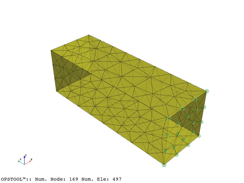
opst.vis.pyvista.set_plot_props(point_size=0, mesh_opacity=0.75)
plotter = opst.vis.pyvista.plot_model()
plotter.show()

Static Scene

Interactive Scene

plotter = opst.vis.pyvista.plot_eigen([1, 9], subplots=True)
plotter.show()

Static Scene

Interactive Scene

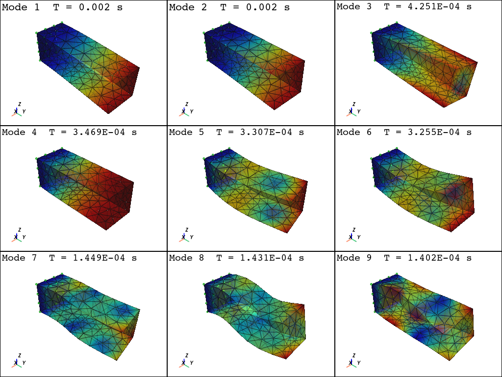
Using DomainModalProperties - Developed by: Massimo Petracca, Guido Camata, ASDEA Software Technology
OPSTOOL™ ::  Eigen data has been saved to G:\opstool\docs\.opstool.output/EigenData-Auto.zarr!

We can apply the load by extracting the elements belonging to surface with tag 27: First, we convert the element to which the surface load is applied to SurfaceLoad Element, and then we can apply the surface load to it:

pressure = -1
load_ele_tags = GMSH2OPS.create_element_cmds(
    ops_ele_type="TriSurfaceLoad",  # OpenSeesPy element type---TriSurfaceLoad
    ops_ele_args=[pressure],  # Additional arguments for the element
    physical_group_names=["Load"],
)

ops.timeSeries("Linear", 1)
ops.pattern("Plain", 1, 1)
ops.eleLoad("-ele", *load_ele_tags, "-type", "-surfaceLoad")

TriSurfaceLoad element - Written: J. A. Abell (UANDES). Inspired by the makers of SurfaceLoad

ops.constraints("Transformation")
ops.numberer("RCM")
ops.system("BandGeneral")
ops.test("NormDispIncr", 1.0e-12, 6, 2)
ops.algorithm("Linear")
ops.integrator("LoadControl", 0.1)
ops.analysis("Static")

ODB = opst.post.CreateODB(odb_tag=1)
for i in range(10):
    ops.analyze(1)
    ODB.fetch_response_step()
ODB.save_response()

OPSTOOL™ ::  All responses data with _odb_tag = 1 saved in G:\opstool\docs\.opstool.output\RespStepData-1.odb!

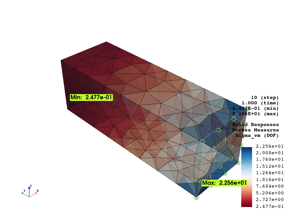
opst.vis.pyvista.set_plot_props(cmap="RdBu", point_size=0.0)

fig = opst.vis.pyvista.plot_unstruct_responses(
    odb_tag=1,
    slides=False,
    ele_type="Solid",
    resp_type="stresses",
    resp_dof="sigma_vm",
)
fig.show()

Static Scene

Interactive Scene

OPSTOOL™ ::  Loading responses data from G:\opstool\docs\.opstool.output\RespStepData-1.odb ...

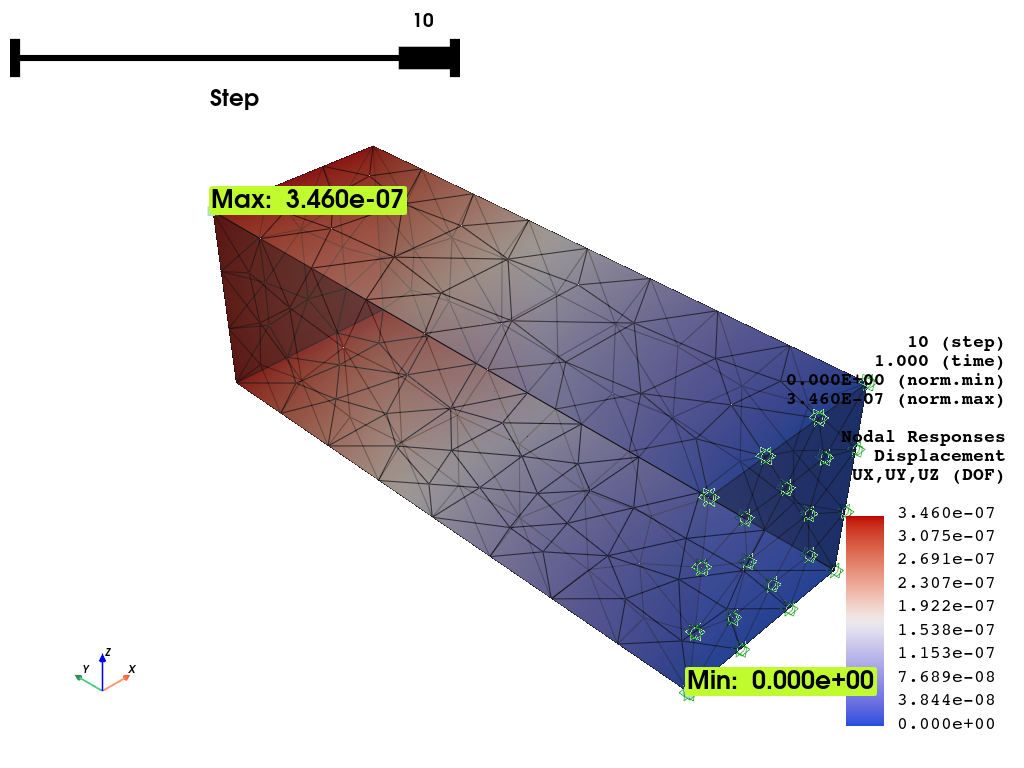
opst.vis.pyvista.set_plot_props(cmap="coolwarm", point_size=0.0)
fig = opst.vis.pyvista.plot_nodal_responses(
    odb_tag=1,
    slides=True,
    resp_type="disp",
    resp_dof=["UX", "UY", "UZ"],
    defo_scale=5,
)
fig.show()

Static Scene

Interactive Scene

OPSTOOL™ ::  Loading responses data from G:\opstool\docs\.opstool.output\RespStepData-1.odb ...