Note
Go to the end to download the full example code.
Modal analysis of a cooling tower
To OpenSeesPy Model
import openseespy.opensees as ops

import opstool as opst
ops.wipe()
ops.model("basic", "-ndm", 3, "-ndf", 6)
E, nu, rho = 2.76e10, 0.166, 2244.0  # Pa, kg/m3
ops.nDMaterial("ElasticIsotropic", 1, E, nu, rho)
secTag = 11
ops.section("PlateFiber", secTag, 1, 0.305)
Read gmsh
GMSH2OPS = opst.pre.Gmsh2OPS(ndm=3, ndf=6)
GMSH2OPS.read_gmsh_file("utils/forma11c.msh")
Info:: 1 Physical Names.
Info:: 1821 Nodes; MaxNodeTag 1821; MinNodeTag 1.
Info:: 2009 Elements; MaxEleTag 2009; MinEleTag 1.
Info:: Geometry Information >>>
53 Entities: 37 Point; 12 Curves; 4 Surfaces; 0 Volumes.

Info:: Physical Groups Information >>>
1 Physical Groups.
Physical Group names: ['Boundary']

Info:: Mesh Information >>>
1821 Nodes; MaxNodeTag 1821; MinNodeTag 1.
1972 Elements; MaxEleTag 2009; MinEleTag 1.
Create OpenSeesPy node commands based on all nodes defined in the GMSH file
node_tags = GMSH2OPS.create_node_cmds()
dim_entity_tags = GMSH2OPS.get_dim_entity_tags()
dim_entity_tags_2D = [item for item in dim_entity_tags if item[0] == 2]
Create OpenSeesPy element commands for specific entities
ele_tags_n4 = GMSH2OPS.create_element_cmds(
    ops_ele_type="ASDShellQ4",  # OpenSeesPy element type
    ops_ele_args=[secTag],  # Additional arguments for the element (e.g., section tag)
    dim_entity_tags=dim_entity_tags_2D,
)
Using ASDShellQ4 - Developed by: Massimo Petracca, Guido Camata, ASDEA Software Technology
Apply boundary conditions
boundary_dim_tags = GMSH2OPS.get_boundary_dim_tags(physical_group_names="Boundary", include_self=True)
print(boundary_dim_tags)
fix_ntags = GMSH2OPS.create_fix_cmds(dim_entity_tags=boundary_dim_tags, dofs=[1] * 6)
removed_node_tags = opst.pre.remove_void_nodes()
[(0, 55), (0, 59), (0, 61), (0, 63), (1, 6), (1, 9), (1, 12), (1, 15)]
Info:: Free nodes with tags [57, 58, 59, 60, 61, 62, 63, 64, 65, 66, 67, 68, 69, 70, 71, 72, 73, 74, 75, 76, 77, 78, 79, 80, 81, 82, 83, 84, 85] have been removed!
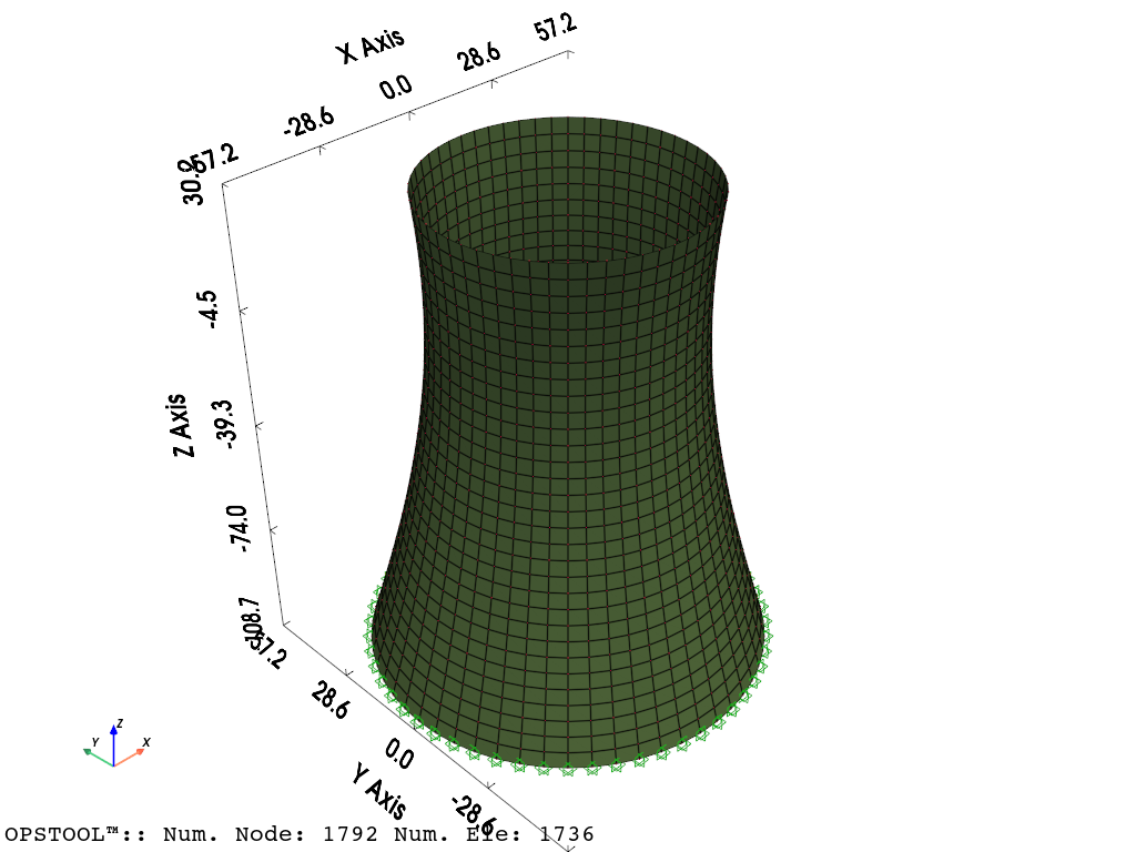
Visualize the model
opst.vis.pyvista.plot_model(show_outline=True).show()
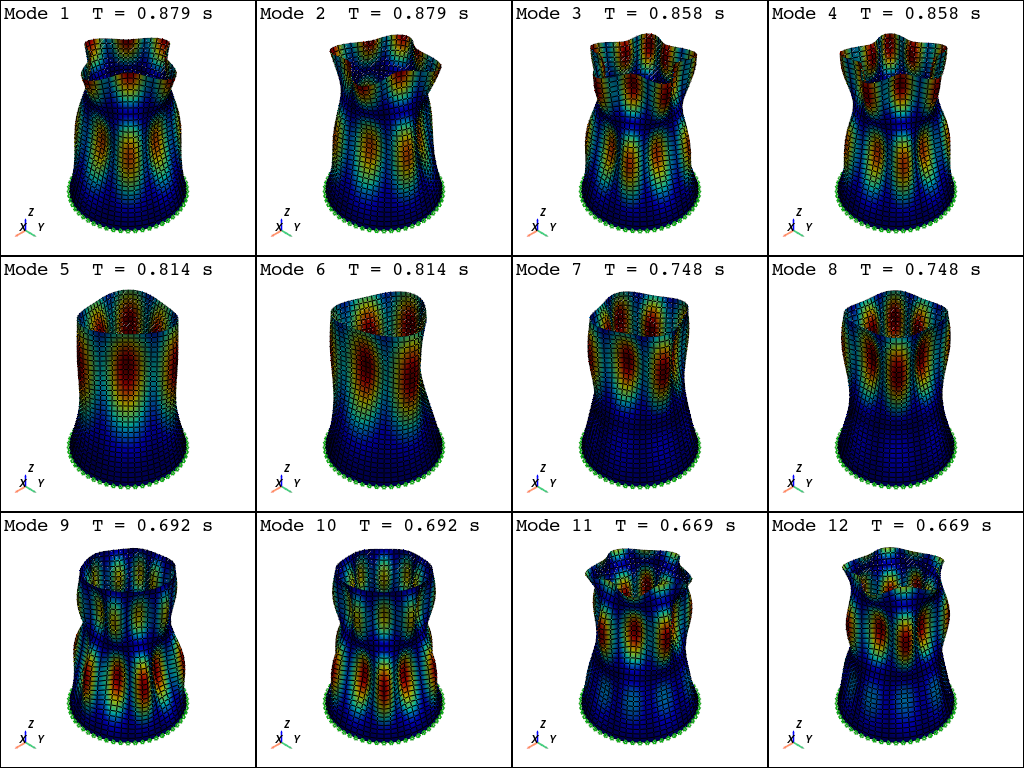
Modal analysis
opst.post.save_eigen_data(odb_tag="eigen", mode_tag=60)
fig = opst.vis.pyvista.plot_eigen(mode_tags=12, odb_tag="eigen", subplots=True)
fig.show()
Using DomainModalProperties - Developed by: Massimo Petracca, Guido Camata, ASDEA Software Technology
OPSTOOL™ ::  Eigen data has been saved to G:\opstool\docs\.opstool.output/EigenData-eigen.zarr!
OPSTOOL™ ::  Loading eigen data from G:\opstool\docs\.opstool.output/EigenData-eigen.zarr ...
Modal Properties
modal_props, eigen_vectors = opst.post.get_eigen_data(odb_tag="eigen")
modal_props = modal_props.to_pandas()
modal_props.head()
OPSTOOL™ :: Loading eigen data from G:\opstool\docs\.opstool.output/EigenData-eigen.zarr ...
modal_props.loc[[1, 47, 48, 60], "eigenFrequency"]
You can compare this with Code-Aster, which uses DKT shell elements. See ~ Model C: Modal analysis of a cooling tower
Gmsh model
You can find modeling instructions at: Creating quadrilateral surface meshes with gmsh
import json
import math

import gmsh
Initialize gmsh
gmsh.initialize()

gmsh.model.add("forma11c_gmsh")
forma11c_profile.json can be downloaded from
here
# Read the profile coordinates
with open("utils/forma11c_profile.json") as file_id:
    coords = json.load(file_id)
Set a default element size
el_size = 1.0

# Add profile points
v_profile = []
for coord in coords:
    v = gmsh.model.occ.addPoint(coord[0], coord[1], coord[2], el_size)
    v_profile.append(v)
Add spline going through profile points
l1 = gmsh.model.occ.addBSpline(v_profile)
# Create copies and rotate
l2 = gmsh.model.occ.copy([(1, l1)])
l3 = gmsh.model.occ.copy([(1, l1)])
l4 = gmsh.model.occ.copy([(1, l1)])

# Rotate the copy
gmsh.model.occ.rotate(l2, 0, 0, 0, 0, 0, 1, math.pi / 2)
gmsh.model.occ.rotate(l3, 0, 0, 0, 0, 0, 1, math.pi)
gmsh.model.occ.rotate(l4, 0, 0, 0, 0, 0, 1, 3 * math.pi / 2)
Sweep the lines
surf1 = gmsh.model.occ.revolve([(1, l1)], 0, 0, 0, 0, 0, 1, math.pi / 2)
surf2 = gmsh.model.occ.revolve(l2, 0, 0, 0, 0, 0, 1, math.pi / 2)
surf3 = gmsh.model.occ.revolve(l3, 0, 0, 0, 0, 0, 1, math.pi / 2)
surf4 = gmsh.model.occ.revolve(l4, 0, 0, 0, 0, 0, 1, math.pi / 2)
Join the surfaces
surf5 = gmsh.model.occ.fragment(surf1, surf2)
surf6 = gmsh.model.occ.fragment(surf3, surf4)
surf7 = gmsh.model.occ.fragment(surf5[0], surf6[0])
gmsh.model.occ.remove_all_duplicates()
gmsh.model.occ.synchronize()
num_nodes_circ = 15
for curve in gmsh.model.occ.getEntities(1):
    gmsh.model.mesh.setTransfiniteCurve(curve[1], num_nodes_circ)
num_nodes_vert = 32
vertical_curves = [7, 10, 13, 17]
for curve in vertical_curves:
    gmsh.model.mesh.setTransfiniteCurve(curve, num_nodes_vert)
for surf in gmsh.model.occ.getEntities(2):
    gmsh.model.mesh.setTransfiniteSurface(surf[1])
gmsh.option.setNumber("Mesh.RecombineAll", 1)
gmsh.option.setNumber("Mesh.RecombinationAlgorithm", 1)
gmsh.option.setNumber("Mesh.Recombine3DLevel", 2)
gmsh.option.setNumber("Mesh.ElementOrder", 1)
Important: Note that we use names to distinguish groups, so please do not overlook this! We use the “Boundary” group to include 4 lines
gmsh.model.addPhysicalGroup(dim=1, tags=[6, 9, 12, 15], tag=1, name="Boundary")
Generate mesh
gmsh.model.mesh.generate(dim=2)
gmsh.option.setNumber("Mesh.SaveAll", 1)
gmsh.write("utils/forma11c.msh")
# gmsh.fltk.run()
Total running time of the script: (0 minutes 4.215 seconds)