Dry single BbarBrick element with pressure dependent material

See PressureDependMultiYield-Example 6 example for more details.

import time

import matplotlib.pyplot as plt
import numpy as np
import openseespy.opensees as ops

import opstool as opst

MODEL CONFIGURATION & PARAMETERS

# ===============================================================
#  MODEL CONFIGURATION & PARAMETERS
#  This script converts the original Tcl model into OpenSeesPy.
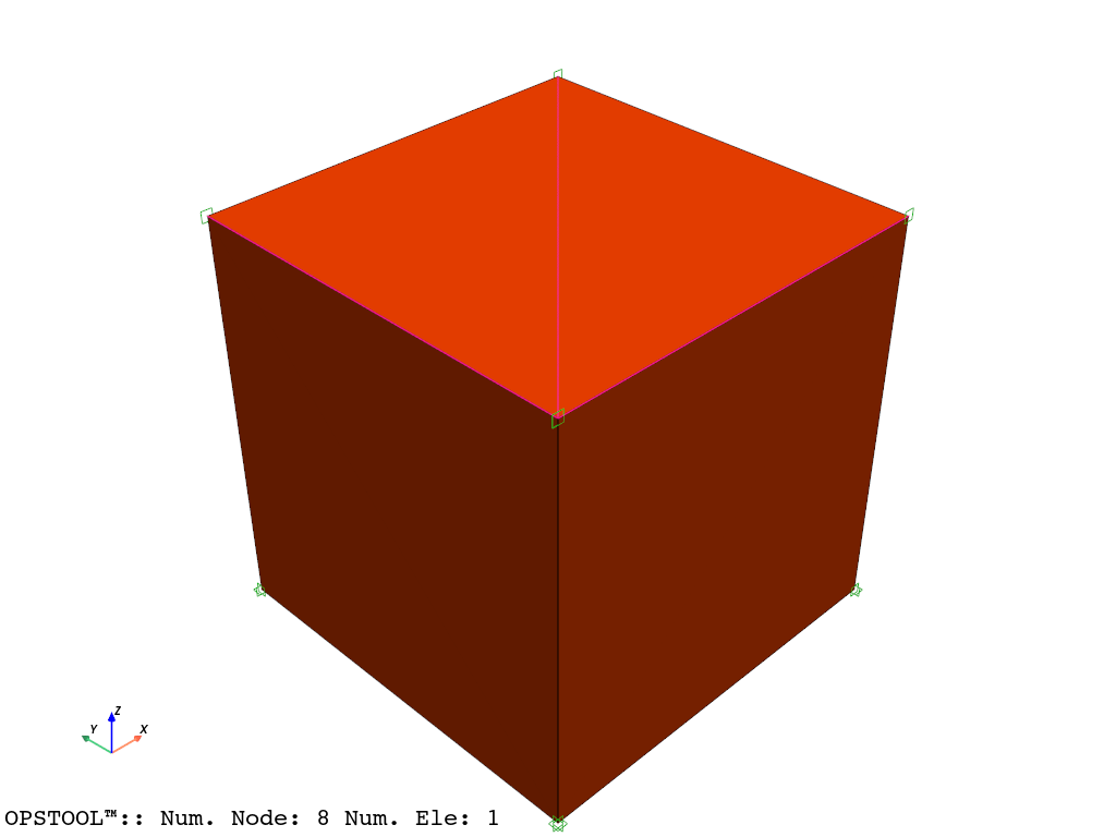
#  A dry bbarBrick element with PressureDependMultiYield material
#  is subjected to 1D sinusoidal base excitation.
# ===============================================================

ops.wipe()

# --- Material & physical parameters ---
friction = 31.40  # Friction angle of the soil
phaseTransform = 26.50  # Phase transformation angle
E1 = 93178.4  # Young's modulus
poisson1 = 0.40  # Poisson’s ratio

# Derived elastic constants
G1 = E1 / (2.0 * (1.0 + poisson1))  # Shear modulus
B1 = E1 / (3.0 * (1.0 - 2.0 * poisson1))  # Bulk modulus

gamma = 0.600  # Newmark gamma parameter

dt = 0.01  # Time step for dynamic analysis
numSteps = 1600  # Number of analysis steps

rhoS = 2.00  # Solid mass density (saturated)
rhoF = 0.00  # Fluid density (dry case → 0)
densityMult = 1.0  # Density multiplier

Bfluid = 2.2e6  # Fluid bulk modulus (unused in dry case)
fluid1 = 1  # Tag for fluid material (not used)
solid1 = 10  # Tag for solid material

accMul = 4.0  # Input acceleration scaling factor

pi = np.pi
inclination = 0.0  # Inclination angle of the element

massProportionalDamping = 0.0
InitStiffnessProportionalDamping = 0.001

# Body forces in global coordinates
bUnitWeightX = (rhoS - 0.0) * 9.81 * np.sin(inclination / 180.0 * pi) * densityMult
bUnitWeightY = 0.0
bUnitWeightZ = -(rhoS - rhoF) * 9.81 * np.cos(inclination / 180.0 * pi)

ndm = 3  # Spatial dimensions
ndf = 3  # Degrees of freedom per node for bricks

# ===============================================================
#  MODEL GENERATION
# ===============================================================
ops.model("Basic", "-ndm", ndm, "-ndf", ndf)

# --- PressureDependMultiYield material definition ---
ops.nDMaterial(
    "PressureDependMultiYield",
    solid1,
    ndm,
    rhoS * densityMult,
    G1,
    B1,
    friction,
    0.1,
    80,
    0.5,
    phaseTransform,
    0.17,
    0.4,
    10,
    10,
    0.015,
    1.0,
)

# --- Nodes of the brick element ---
ops.node(1, 0, 0, 0)
ops.node(2, 0, 0, 1)
ops.node(3, 0, 1, 0)
ops.node(4, 0, 1, 1)
ops.node(5, 1, 0, 0)
ops.node(6, 1, 0, 1)
ops.node(7, 1, 1, 0)
ops.node(8, 1, 1, 1)

# --- bbarBrick element ---
ops.element("bbarBrick", 1, 1, 5, 7, 3, 2, 6, 8, 4, solid1, bUnitWeightX, bUnitWeightY, bUnitWeightZ)

# Initially, set the material to "elastic stage"
ops.updateMaterialStage("-material", solid1, "-stage", 0)

# ===============================================================
#  BOUNDARY CONDITIONS
# ===============================================================
# Note: Brick elements use 3 DOFs (UX, UY, UZ). Rotations are not present.

ops.fix(1, 1, 1, 1)
ops.fix(2, 0, 1, 0)
ops.fix(3, 1, 1, 1)
ops.fix(4, 0, 1, 0)
ops.fix(5, 1, 1, 1)
ops.fix(6, 0, 1, 0)
ops.fix(7, 1, 1, 1)
ops.fix(8, 0, 1, 0)

# Equal DOF constraints (to tie boundary nodes)
ops.equalDOF(2, 4, 1, 3)
ops.equalDOF(2, 6, 1, 3)
ops.equalDOF(2, 8, 1, 3)

fig = opst.vis.pyvista.plot_model()
fig.show()

Static Scene

Interactive Scene

ANALYSIS

# ===============================================================
#  STATIC GRAVITY ANALYSIS (Elastic stage)
# ===============================================================
ops.system("ProfileSPD")
ops.test("NormDispIncr", 1e-10, 25, 2)
ops.constraints("Transformation")
ops.integrator("LoadControl", 1.0, 1, 1, 1)
ops.algorithm("Newton")
ops.numberer("RCM")
ops.analysis("Static")

ops.analyze(2)

# ===============================================================
#  SWITCH MATERIAL TO PLASTIC STAGE
# ===============================================================
ops.updateMaterialStage("-material", solid1, "-stage", 1)
# ops.updateMaterials("-material", solid1, "bulkModulus", G1 * 2.0 / 3.0)
ops.setParameter("-val", G1 * 2.0 / 3.0, "-ele", *[1], "bulkModulus")

ops.analyze(2)

# Reset time for dynamic analysis
ops.setTime(0.0)
ops.wipeAnalysis()


# ===============================================================
#  DYNAMIC ANALYSIS CONFIGURATION
# ===============================================================
# Sinusoidal base excitation: Sine(start, end, period)
ops.timeSeries("Sine", 1, 0.0, 10.0, 1.0, "-factor", accMul)
ops.pattern("UniformExcitation", 1, 1, "-accel", 1)

ops.rayleigh(massProportionalDamping, 0.0, InitStiffnessProportionalDamping, 0.0)

beta = (gamma + 0.5) ** 2 / 4.0
ops.integrator("Newmark", gamma, beta)

ops.constraints("Penalty", 1e18, 1e18)
ops.test("NormDispIncr", 1e-10, 25, 0)
ops.algorithm("ModifiedNewton")
ops.system("ProfileSPD")
ops.numberer("Plain")
ops.analysis("VariableTransient")

CTestNormDispIncr::test() - iteration: 2 current Norm: 1.6125e-20 (max: 1e-10, Norm deltaR: 1.16573e-15)
CTestNormDispIncr::test() - iteration: 1 current Norm: 5.83836e-21 (max: 1e-10, Norm deltaR: 3.88578e-16)
CTestNormDispIncr::test() - iteration: 1 current Norm: 7.62496e-21 (max: 1e-10, Norm deltaR: 7.59948e-14)
CTestNormDispIncr::test() - iteration: 1 current Norm: 1.31009e-18 (max: 1e-10, Norm deltaR: 6.71685e-15)

RUN TIME-HISTORY ANALYSIS

startT = time.time()
ODB = opst.post.CreateODB(
    odb_tag=1,
    compute_mechanical_measures=True,
    project_gauss_to_nodes="copy",  # "extrapolate", "copy", "average"
)
for _ in range(numSteps):
    ops.analyze(1, dt)
    ODB.fetch_response_step()
ODB.save_response()
endT = time.time()

print(f"Execution time: {endT - startT:.3f} seconds.")

OPSTOOL™ ::  All responses data with _odb_tag = 1 saved in G:\opstool\docs\.opstool.output\RespStepData-1.odb!
Execution time: 1.940 seconds.

POST-PROCESSING

Nodal Response

node_resp = opst.post.get_nodal_responses(odb_tag=1)
print(node_resp)

OPSTOOL™ ::  Loading all response data from G:\opstool\docs\.opstool.output\RespStepData-1.odb ...
<xarray.DatasetView> Size: 2MB
Dimensions:             (time: 1601, nodeTags: 8, DOFs: 6)
Coordinates:
  * time                (time) float32 6kB 0.0 0.01 0.02 ... 15.98 15.99 16.0
  * nodeTags            (nodeTags) int64 64B 1 2 3 4 5 6 7 8
  * DOFs                (DOFs) <U2 48B 'UX' 'UY' 'UZ' 'RX' 'RY' 'RZ'
Data variables:
    accel               (time, nodeTags, DOFs) float32 307kB 0.0 0.0 ... 0.0 0.0
    disp                (time, nodeTags, DOFs) float32 307kB 0.0 0.0 ... 0.0 0.0
    pressure            (time, nodeTags) float32 51kB 0.0 0.0 0.0 ... 0.0 0.0
    rayleighForces      (time, nodeTags, DOFs) float32 307kB 0.0 0.0 ... 0.0 0.0
    reaction            (time, nodeTags, DOFs) float32 307kB 1.635 1.635 ... 0.0
    reactionIncInertia  (time, nodeTags, DOFs) float32 307kB 1.635 1.635 ... 0.0
    vel                 (time, nodeTags, DOFs) float32 307kB 0.0 0.0 ... 0.0 0.0
Attributes:
    UX:       Displacement in X direction
    UY:       Displacement in Y direction
    UZ:       Displacement in Z direction
    RX:       Rotation about X axis
    RY:       Rotation about Y axis
    RZ:       Rotation about Z axis

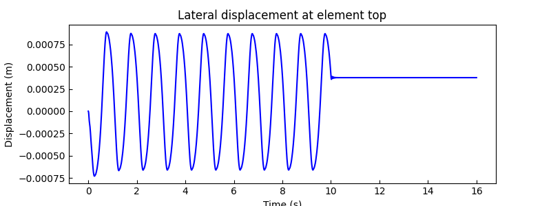
node 3 displacement relative to node 1

disp1 = node_resp["disp"].sel(nodeTags=1, DOFs="UX")
disp8 = node_resp["disp"].sel(nodeTags=8, DOFs="UX")
times = node_resp["time"].data

fig, ax = plt.subplots(1, 1, figsize=(8, 3))
ax.plot(times, disp8 - disp1, "b")
ax.set_title("Lateral displacement at element top")
ax.set_xlabel("Time (s)")
ax.set_ylabel("Displacement (m)")
plt.show()

Elemental response

ele_resp = opst.post.get_element_responses(odb_tag=1, ele_type="brick")
print("Data Variables in Element Responses:", ele_resp.data_vars)

OPSTOOL™ ::  Loading brick response data from G:\opstool\docs\.opstool.output\RespStepData-1.odb ...
Data Variables in Element Responses: Data variables:
    PorePressureAtNodes    (time, nodeTags) float64 102kB 0.0 0.0 ... 0.0 0.0
    Strains                (time, eleTags, GaussPoints, strainDOFs) float32 307kB ...
    StrainsAtNodes         (time, nodeTags, strainDOFs) float32 307kB 5.717e-...
    StrainsAtNodesErr      (time, nodeTags, strainDOFs) float32 307kB 0.0 ......
    StressAtNodesErr       (time, nodeTags, stressDOFs) float32 359kB 0.0 ......
    Stresses               (time, eleTags, GaussPoints, stressDOFs) float32 359kB ...
    StressesAtNodes        (time, nodeTags, stressDOFs) float32 359kB -6.54 ....
    StressMeasures         (time, eleTags, GaussPoints, measures) float32 359kB ...
    StressMeasuresAtNodes  (time, nodeTags, measures) float32 359kB -6.54 ......

print(ele_resp.coords)

Coordinates:
  * time         (time) float32 6kB 0.0 0.01 0.02 0.03 ... 15.98 15.99 16.0
  * nodeTags     (nodeTags) int64 64B 1 5 7 3 2 6 8 4
  * eleTags      (eleTags) int64 8B 1
  * GaussPoints  (GaussPoints) int64 64B 1 2 3 4 5 6 7 8
  * strainDOFs   (strainDOFs) <U5 120B 'eps11' 'eps22' ... 'eps23' 'eps13'
  * stressDOFs   (stressDOFs) <U7 196B 'sigma11' 'sigma22' ... 'para#1'
  * measures     (measures) <U9 252B 'p1' 'p2' 'p3' ... 'tau_oct' 'tau_max'

for key, value in ele_resp.attrs.items():
    print(f"{key}: {value}")

sigma11, sigma22, sigma33: Normal stress (strain) along x, y, z.
sigma12, sigma23, sigma13: Shear stress (strain).
para#i: The additional output of stress, which is useful for some elements, such as * eta_r * for some u-p elements. eta_r--Ratio between the shear (deviatoric) stress and peak shear strength at the current confinement.
p1, p2, p3: Principal stresses, p3=0 for 2D plane stress condition, p3!=0 for 3D plane strain condition.
sigma_vm: Von Mises stress.
tau_max: Maximum shear stress, 0.5*(p1-p3).
sigma_oct: Octahedral normal stress, (p1+p2+p3)/3.
tau_oct: Octahedral shear stress, sqrt(2/3*J2).
sigma_mohr_coulomb_sy_eq: Mohr-Coulomb equivalent stress (using tensile and compressive strengths).
sigma_mohr_coulomb_sy_intensity: Mohr-Coulomb intensity (using tensile and compressive strengths).
sigma_mohr_coulomb_c_phi_eq: Mohr-Coulomb equivalent stress (using cohesion and friction angle).
sigma_mohr_coulomb_c_phi_intensity: Mohr-Coulomb intensity (using cohesion and friction angle).
sigma_drucker_prager_sy_eq: Drucker-Prager equivalent stress (using tensile and compressive strengths).
sigma_drucker_prager_sy_intensity: Drucker-Prager intensity (using tensile and compressive strengths).
sigma_drucker_prager_c_phi_eq: Drucker-Prager equivalent stress (using cohesion and friction angle).
sigma_drucker_prager_c_phi_intensity: Drucker-Prager intensity (using cohesion and friction angle).

Gauss point responses

sigma11 = ele_resp["Stresses"].sel(stressDOFs="sigma11", eleTags=1)
sigma22 = ele_resp["Stresses"].sel(stressDOFs="sigma22", eleTags=1)
sigma33 = ele_resp["Stresses"].sel(stressDOFs="sigma33", eleTags=1)
sigma12 = ele_resp["Stresses"].sel(stressDOFs="sigma12", eleTags=1)
sigma13 = ele_resp["Stresses"].sel(stressDOFs="sigma13", eleTags=1)
sigma23 = ele_resp["Stresses"].sel(stressDOFs="sigma23", eleTags=1)

Calculate confinement p and deviatoric stress q

po = ele_resp["StressMeasures"].sel(measures="sigma_oct", eleTags=1)
qo = ele_resp["StressMeasures"].sel(measures="tau_oct", eleTags=1)
print(qo)

<xarray.DataArray 'StressMeasures' (time: 1601, GaussPoints: 8)> Size: 51kB
array([[1.541493  , 1.541493  , 1.541493  , ..., 1.541493  , 1.541493  ,
        1.541493  ],
       [1.541422  , 1.541422  , 1.541422  , ..., 1.541422  , 1.541422  ,
        1.541422  ],
       [1.5525209 , 1.5525209 , 1.5525209 , ..., 1.5525209 , 1.5525209 ,
        1.5525209 ],
       ...,
       [0.36760953, 0.36760953, 0.36760953, ..., 0.36760953, 0.36760953,
        0.36760953],
       [0.36760953, 0.36760953, 0.36760953, ..., 0.36760953, 0.36760953,
        0.36760953],
       [0.36760953, 0.36760953, 0.36760953, ..., 0.36760953, 0.36760953,
        0.36760953]], shape=(1601, 8), dtype=float32)
Coordinates:
  * time         (time) float32 6kB 0.0 0.01 0.02 0.03 ... 15.98 15.99 16.0
  * GaussPoints  (GaussPoints) int64 64B 1 2 3 4 5 6 7 8
    eleTags      int64 8B 1
    measures     <U9 36B 'tau_oct'

strain components

eps11 = ele_resp["Strains"].sel(strainDOFs="eps11", eleTags=1)
eps22 = ele_resp["Strains"].sel(strainDOFs="eps22", eleTags=1)
eps33 = ele_resp["Strains"].sel(strainDOFs="eps33", eleTags=1)
eps12 = ele_resp["Strains"].sel(strainDOFs="eps12", eleTags=1)
eps13 = ele_resp["Strains"].sel(strainDOFs="eps13", eleTags=1)
eps23 = ele_resp["Strains"].sel(strainDOFs="eps23", eleTags=1)

eps13_ele1_1 = eps13.sel(GaussPoints=1)
sigma13_ele1_1 = sigma13.sel(GaussPoints=1)
po_ele1_1 = po.sel(GaussPoints=1)
qo_ele1_1 = qo.sel(GaussPoints=1) * np.sign(sigma13_ele1_1)

fig, axs = plt.subplots(1, 2, figsize=(10, 3))
axs[0].plot(eps13_ele1_1, sigma13_ele1_1, "b")
axs[0].set_title("shear stress $\\tau_{xz}$ VS. shear strain $\\epsilon_{xz}$ \n at integration point 1")
axs[0].set_xlabel(r"Shear strain $\epsilon_{xz}$")
axs[0].set_ylabel(r"Shear stress $\tau_{xz}$ (kPa)")
axs[1].plot(-po_ele1_1, qo_ele1_1, "r")
axs[1].set_title("confinement p VS. deviatoric stress q \n at integration point 1")
axs[1].set_xlabel("confinement p (kPa)")
axs[1].set_ylabel("q (kPa)")
plt.show()

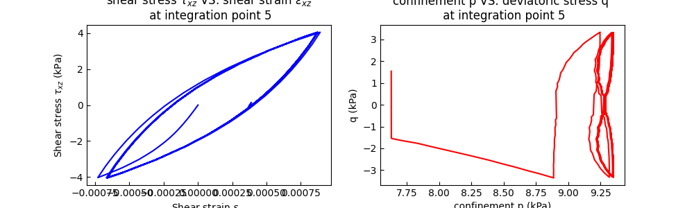
eps13_ele1_1 = eps13.sel(GaussPoints=5)
sigma13_ele1_1 = sigma13.sel(GaussPoints=5)
po_ele1_1 = po.sel(GaussPoints=5)
qo_ele1_1 = qo.sel(GaussPoints=5) * np.sign(sigma13_ele1_1)

fig, axs = plt.subplots(1, 2, figsize=(10, 3))
axs[0].plot(eps13_ele1_1, sigma13_ele1_1, "b")
axs[0].set_title("shear stress $\\tau_{xz}$ VS. shear strain $\\epsilon_{xz}$ \n at integration point 5")
axs[0].set_xlabel(r"Shear strain $\epsilon_{xz}$")
axs[0].set_ylabel(r"Shear stress $\tau_{xz}$ (kPa)")
axs[1].plot(-po_ele1_1, qo_ele1_1, "r")
axs[1].set_title("confinement p VS. deviatoric stress q \n at integration point 5")
axs[1].set_xlabel("confinement p (kPa)")
axs[1].set_ylabel("q (kPa)")
plt.show()