Moment Curvature Analysis of Section#
- class opstool.analysis.MomentCurvature(sec_tag, axial_force=0)[source]#
Moment-Curvature Analysis for Fiber Section in OpenSeesPy.
Parameters#
- sec_tagint,
The previously defined section Tag.
- axial_forcefloat, optional
Axial load, compression is negative, by default 0
- analyze(axis='y', max_phi=0.25, incr_phi=0.0001, limit_peak_ratio=0.8, smart_analyze=True, debug=False)[source]#
Performing Moment-Curvature Analysis.
Parameters#
- axisstr, optional, “y” or “z”
The axis of the section to be analyzed, by default “y”.
- max_phifloat, optional
The maximum curvature to analyze, by default 1.0.
- incr_phifloat, optional
Curvature analysis increment, by default 1e-4.
- limit_peak_ratiofloat, optional
A ratio of the moment intensity after the peak used to stop the analysis., by default 0.8, i.e. a 20% drop after peak.
- smart_analyzebool, optional
Whether to use smart analysis options, by default True.
- debug: bool, optional
Whether to use debug mode when smart analysis is True, by default False.
Note
The termination of the analysis depends on whichever reaches max_phi or post_peak_ratio first.
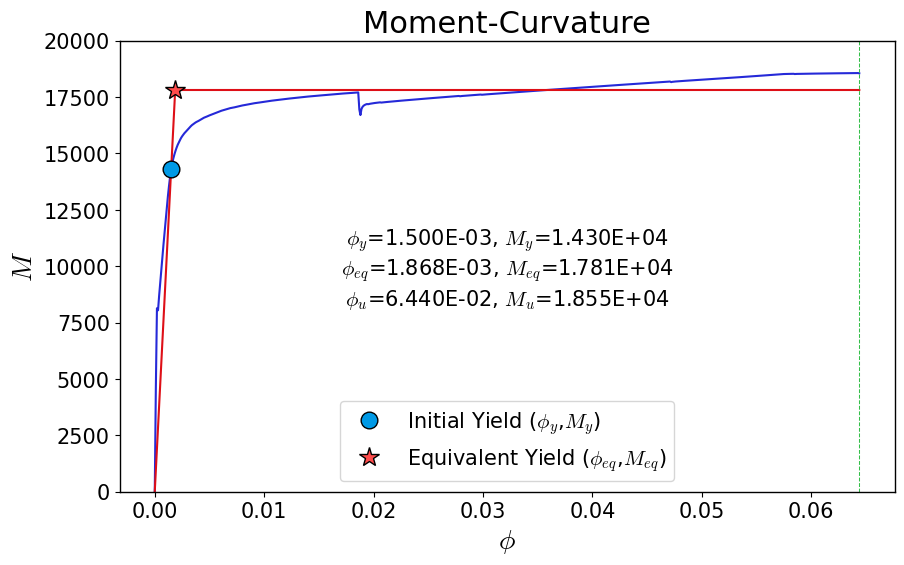
- bilinearize(phiy, My, phiu, plot=False, return_ax=False)[source]#
Bilinear Approximation of Moment-Curvature Relation.
Parameters#
- phiyfloat
The initial yield curvature.
- Myfloat
The initial yield moment.
- phiufloat
The limit curvature.
- plotbool, optional
If True, plot the bilinear approximation, by default False.
- return_ax: bool, default=False
If True, return the axes for the plot of matplotlib.
Returns#
- (float, float)
(Equivalent Curvature, Equivalent Moment)
- get_M_phi()[source]#
Get the moment and curvature array.
Returns#
- (1D array-like, 1D array-like)
(Curvature array, Moment array)
- get_fiber_data()[source]#
All fiber data.
Returns#
- Shape-(n,m,6) Array.
n is the length of analysis steps, m is the fiber number, 6 contain (“yCoord”, “zCoord”, “area”, ‘mat’, “stress”, “strain”)
- get_limit_state(matTag=1, threshold=0, peak_drop=False)[source]#
Get the curvature and moment corresponding to a certain limit state.
Parameters#
- matTagint, optional
The OpenSeesPy material Tag used to determine the limit state., by default 1
- thresholdfloat, optional
The strain threshold used to determine the limit state by material matTag, by default 0
- peak_dropUnion[float, bool], optional
If True, A default 20% drop from the peak value of the moment will be used as the limit state; If float in [0, 1], this means that the ratio of ultimate strength to peak value is specified by this value, for example, peak_drop = 0.3, the ultimate strength = 0.7 * peak. matTag and threshold are not needed, by default False.
Returns#
- (float, float)
(Limit Curvature, Limit Moment)
Example#
import opstool as opst
import openseespy.opensees as ops

ops.wipe()
ops.model('basic', '-ndm', 3, '-ndf', 6)
Note that you need to set the model to 6DOF in 3D, because the program takes two axes into account.
Create any opensees material yourself as follows:
# materials
Ec = 3.55E+7
Vc = 0.2
Gc = 0.5 * Ec / (1 + Vc)
fc = -32.4E+3
ec = -2000.0E-6
ecu = 2.1 * ec
ft = 2.64E+3
et = 107E-6
fccore = -40.6e+3
eccore = -4079e-6
ecucore = -0.0144

Fys = 400.E+3
Fus = 530.E+3
Es = 2.0E+8
eps_sh = 0.0074
eps_ult = 0.095
Esh = (Fus - Fys) / (eps_ult - eps_sh)
bs = 0.01

matTagC = 1
matTagCCore = 2
matTagS = 3
ops.uniaxialMaterial('Concrete04', matTagC, fc, ec, ecu, Ec, ft, et)
ops.uniaxialMaterial('Concrete04', matTagCCore, fccore,
                     eccore, ecucore, Ec, ft, et)  # for core
ops.uniaxialMaterial('ReinforcingSteel', matTagS, Fys,
                     Fus, Es, Esh, eps_sh, eps_ult)
Create the section mesh by **opstool**(see SecMesh):
outlines = [[0, 0], [2, 0], [2, 2], [0, 2]]
coverlines = opst.offset(outlines, d=0.05)
cover = opst.add_polygon(outlines, holes=[coverlines])
holelines = [[0.5, 0.5], [1.5, 0.5], [1.5, 1.5], [0.5, 1.5]]
core = opst.add_polygon(coverlines, holes=[holelines])
sec = opst.SecMesh()
sec.assign_group(dict(cover=cover, core=core))
sec.assign_mesh_size(dict(cover=0.02, core=0.05))
sec.assign_group_color(dict(cover="gray", core="green"))
sec.assign_ops_matTag(dict(cover=matTagC, core=matTagCCore))
sec.mesh()
# add rebars
rebars = opst.Rebars()
rebar_lines1 = opst.offset(outlines, d=0.05 + 0.032 / 2)
rebars.add_rebar_line(
   points=rebar_lines1, dia=0.02, gap=0.1, color="red",
   matTag=matTagS,
)
sec.add_rebars(rebars)
# sec.get_sec_props(display_results=False, plot_centroids=False)
sec.centring()
# sec.rotate(45)
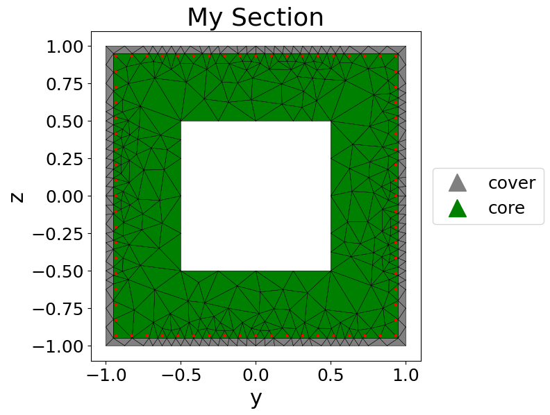
Plot the section mesh:
sec.view(fill=True, engine='matplotlib', save_html=None, on_notebook=True)
Generate the OpenSeesPy commands to the domin(important!)
sec.opspy_cmds(secTag=1, GJ=100000)
Now you can perform a moment-curvature analysis:
mc = opst.MomentCurvature(sec_tag=1, axial_force=-10000)
mc.analyze(axis='y')
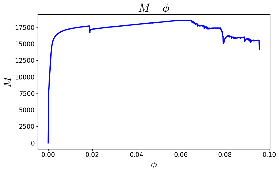
Plot the moment-curvature relationship:
mc.plot_M_phi()
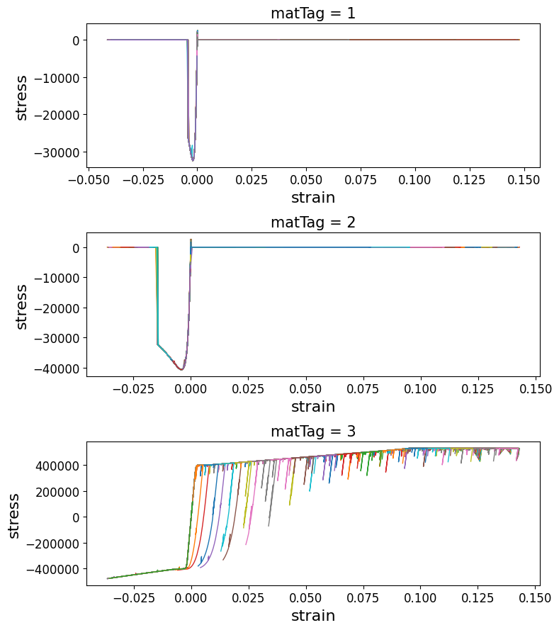
Plot all fiber stress-strain responses:
mc.plot_fiber_responses()
Extract limit state points based on fiber strain thresholds or other criteria.
# Tensile steel fibers yield (strain=2e-3) for the first time
phiy, My = mc.get_limit_state(matTag=matTagS,
                              threshold=2e-3,)
# The concrete fiber in the confined area reaches the ultimate compressive strain 0.0144
phiu, Mu = mc.get_limit_state(matTag=matTagCCore,
                              threshold=-0.0144,
                              peak_drop=False
                              )
# or use peak_drop
# phiu, Mu = mc.get_limit_state(matTag=matTagCCore,
#                               threshold=-0.0144,
#                               peak_drop=0.2
#                              )
Equivalent linearization according to area:
phi_eq, M_eq = mc.bilinearize(phiy, My, phiu, plot=True)