Truss element Response

import openseespy.opensees as ops
import opstool as opst
import matplotlib.pyplot as plt
%matplotlib inline

ops.wipe()
ops.model("basic", "-ndm", 2, "-ndf", 2)
# variables
A = 4.0
E = 29000.0
alpha = 0.05
sY = 36.0
udisp = 2.5
Nsteps = 1000
Px = 160.0
Py = 0.0
# create nodes
ops.node(1, 0.0, 0.0)
ops.node(2, 72.0, 0.0)
ops.node(3, 168.0, 0.0)
ops.node(4, 48.0, 144.0)
# set boundary condition
ops.fix(1, 1, 1)
ops.fix(2, 1, 1)
ops.fix(3, 1, 1)
# define materials
ops.uniaxialMaterial("Hardening", 1, E, sY, 0.0, alpha / (1 - alpha) * E)
# define elements
ops.element("Truss", 1, 1, 4, A, 1)
ops.element("Truss", 2, 2, 4, A, 1)
ops.element("Truss", 3, 3, 4, A, 1)
# create TimeSeries
ops.timeSeries("Linear", 1)
# create a plain load pattern
ops.pattern("Plain", 1, 1)
# Create the nodal load
ops.load(4, Px, Py)

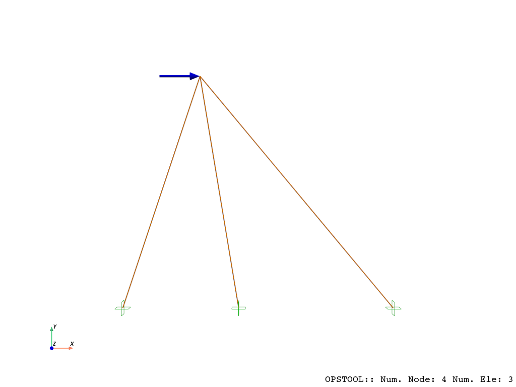
# plot
opst.vis.pyvista.set_plot_props(notebook=True)
fig = opst.vis.pyvista.plot_model(show_nodal_loads=True, load_scale=3, bc_scale=5)
fig.show(jupyter_backend="static")

OPSTOOL ::  Model data has been saved to _OPSTOOL_ODB/ModelData-None.nc!

Result Saving

ops.system("BandGeneral")
ops.constraints("Transformation")
ops.numberer("RCM")
ops.test("NormDispIncr", 1.0e-12, 10, 3)
ops.algorithm("Newton")
ops.integrator("LoadControl", 1.0 / Nsteps)
ops.analysis("Static")

opstool allows us to save the data at each step of the analysis! First, we create a database class using opstool.post.CreateODB, and then, during each step of the analysis, we call its method .fetch_response_step to retrieve the data for the current step. Once all the analysis steps are completed, we use the .save_response method to save the data in one go.

ODB = opst.post.CreateODB(odb_tag=1)
for i in range(Nsteps):
    ops.analyze(1)
    ODB.fetch_response_step()
ODB.save_response()

Result Reading

The provided function opstool.post.get_element_responses() make it easy to read element responses.

ele_type="Truss" is used to specify extracting the response of frame elements.

all_resp = opst.post.get_element_responses(odb_tag=1, ele_type="Truss")

OPSTOOL ::  Loading response data from _OPSTOOL_ODB/RespStepData-1.nc ...

The result is an xarray DataSet object, and we can access the associated DataArray objects through .data_vars.

all_resp.data_vars

Data variables:
    axialForce  (time, eleTags) float64 24kB ...
    axialDefo   (time, eleTags) float64 24kB ...
    Stress      (time, eleTags) float64 24kB ...
    Strain      (time, eleTags) float64 24kB ...

The variable names, along with their dimensions and coordinates, are displayed above. The first two represent the axial force and deformation of the truss element, while the latter refers to the stress and strain of the material in its cross-section.

all_resp["axialForce"]

<xarray.DataArray 'axialForce' (time: 1001, eleTags: 3)> Size: 24kB
[3003 values with dtype=float64]
Coordinates:
  * eleTags  (eleTags) int32 12B 1 2 3
  * time     (time) float64 8kB 0.0 0.001 0.002 0.003 ... 0.997 0.998 0.999 1.0

xarray.DataArray

'axialForce'

• time: 1001
• eleTags: 3

• ...

  [3003 values with dtype=float64]

• Coordinates: (2)
  • eleTags
    (eleTags)
    int32
    1 2 3

    array([1, 2, 3])

  • time
    (time)
    float64
    0.0 0.001 0.002 ... 0.998 0.999 1.0

    array([0.00e+00, 1.00e-03, 2.00e-03, ..., 9.98e-01, 9.99e-01, 1.00e+00])

• Indexes: (2)
  • eleTags
    PandasIndex

    PandasIndex(Index([1, 2, 3], dtype='int32', name='eleTags'))

  • time
    PandasIndex

    PandasIndex(Index([                 0.0,                0.001,                0.002,
                          0.003,                0.004,                0.005,
                          0.006,                0.007,                0.008,
           0.009000000000000001,
           ...
             0.9910000000000008,   0.9920000000000008,   0.9930000000000008,
             0.9940000000000008,   0.9950000000000008,   0.9960000000000008,
             0.9970000000000008,   0.9980000000000008,   0.9990000000000008,
             1.0000000000000007],
          dtype='float64', name='time', length=1001))

• Attributes: (0)

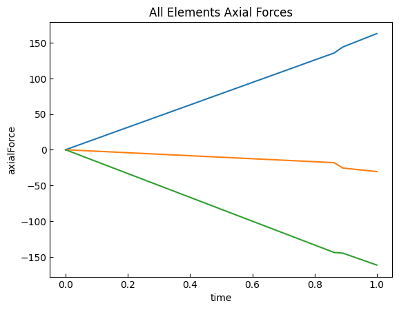
all_resp["axialForce"].plot.line(
    x="time",
    add_legend=False,
)
plt.title("All Elements Axial Forces")
plt.show()

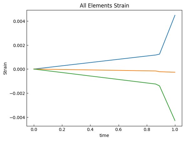
all_resp["Strain"].plot.line(
    x="time",
    add_legend=False,
)
plt.title("All Elements Strain")
plt.show()

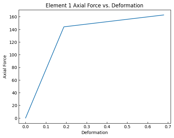
axialForce = opst.post.get_element_responses(
    odb_tag=1, ele_type="Truss", resp_type="axialForce"
)
axialDefo = opst.post.get_element_responses(
    odb_tag=1, ele_type="Truss", resp_type="axialDefo"
)

plt.plot(axialDefo.sel(eleTags=1), axialForce.sel(eleTags=1))
plt.title("Element 1 Axial Force vs. Deformation")
plt.xlabel("Deformation")
plt.ylabel("Axial Force")
plt.show()

OPSTOOL ::  Loading response data from _OPSTOOL_ODB/RespStepData-1.nc ...

OPSTOOL ::  Loading response data from _OPSTOOL_ODB/RespStepData-1.nc ...