Brick element Response
[1]:
import numpy as np
import openseespy.opensees as ops
import opstool as opst
import matplotlib.pyplot as plt
[2]:
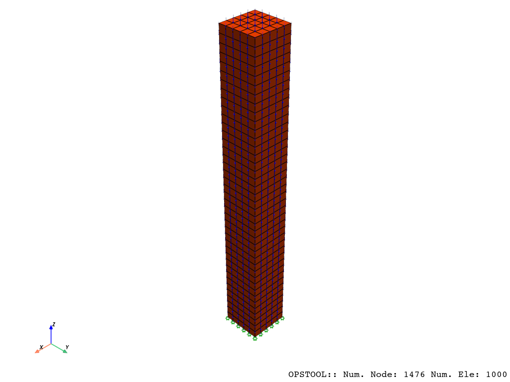
opst.load_ops_examples("Pier-Brick")  # or your model code here

# add beam loads
ops.timeSeries("Linear", 1)
ops.pattern("Plain", 1, 1)
opst.pre.gen_grav_load(direction="z", factor=-9.81)


# plot
opst.vis.pyvista.set_plot_props(notebook=True)
fig = opst.vis.pyvista.plot_model(show_nodal_loads=True)
fig.show(jupyter_backend="static")
OPSTOOL :: Model data has been saved to _OPSTOOL_ODB/ModelData-None.nc!
Result Saving
[3]:
ops.system("BandGeneral")
# Create the constraint handler, the transformation method
ops.constraints("Transformation")
# Create the DOF numberer, the reverse Cuthill-McKee algorithm
ops.numberer("RCM")
# Create the convergence test, the norm of the residual with a tolerance of
# 1e-12 and a max number of iterations of 10
ops.test("NormDispIncr", 1.0e-12, 10, 3)
# Create the solution algorithm, a Newton-Raphson algorithm
ops.algorithm("Newton")
# Create the integration scheme, the LoadControl scheme using steps of 0.1
ops.integrator("LoadControl", 0.1)
# Create the analysis object
ops.analysis("Static")
opstool allows us to save the data at each step of the analysis!
First, we create a database class using opstool.post.CreateODB, and then, during each step of the analysis, we call its method .fetch_response_step to retrieve the data for the current step.
Once all the analysis steps are completed, we use the .save_response method to save the data in one go.
[4]:
ODB = opst.post.CreateODB(odb_tag=1)
for i in range(10):
    ops.analyze(1)
    ODB.fetch_response_step()
ODB.save_response()
OPSTOOL :: All responses data with odb_tag = 1 saved in _OPSTOOL_ODB/RespStepData-1.nc!
Result Reading
The provided function opstool.post.get_element_responses() make it easy to read element responses.
ele_type="Shell" is used to specify extracting the response of shell elements.
[5]:
all_resp = opst.post.get_element_responses(odb_tag=1, ele_type="Brick")
OPSTOOL :: Loading response data from _OPSTOOL_ODB/RespStepData-1.nc ...
The result is an xarray DataSet object, and we can access the associated DataArray objects through .data_vars.
[6]:
all_resp.data_vars
[6]:
Data variables:
    Stresses  (time, eleTags, GaussPoints, DOFs) float64 9MB ...
    Strains   (time, eleTags, GaussPoints, DOFs) float64 9MB ...
Stresses and Strains refer to the stress and strain at the Gauss points. Stress and strain consist of six components aligned with the global coordinate system, as well as additional stress measures:
[7]:
all_resp.DOFs.data
[7]:
array(['sigma11', 'sigma22', 'sigma33', 'sigma12', 'sigma23', 'sigma13',
       'p1', 'p2', 'p3', 'sigma_vm', 'tau_max', 'sigma_oct', 'tau_oct'],
      dtype='<U9')
[8]:
all_resp.attrs # attributes
[8]:
{'sigma11, sigma22, sigma33': 'Normal stress (strain) along x, y, z.',
 'sigma12, sigma23, sigma13': 'Shear stress (strain).',
 'p1, p2, p3': 'Principal stresses (strains).',
 'sigma_vm': 'Von Mises stress.',
 'tau_max': 'Maximum shear stress (strains).',
 'sigma_oct': 'Octahedral normal stress (strains).',
 'tau_oct': 'Octahedral shear stress (strains).'}
Below, we retrieve the stress and strain data, which is a 4D array. The dimensions are, in order, (‘time’, ‘eleTags’, ‘GaussPoints’, ‘DOFs’), and we can conveniently retrieve data based on these dimensions and their coordinates.
[9]:
stresses = all_resp["Stresses"]
strains = all_resp["Strains"]
print(stresses)
print("=" * 100)
print(strains)
print("=" * 100)
print(stresses.dims)
<xarray.DataArray 'Stresses' (time: 11, eleTags: 1000, GaussPoints: 8, DOFs: 13)> Size: 9MB
[1144000 values with dtype=float64]
Coordinates:
  * eleTags      (eleTags) int32 4kB 1 2 3 4 5 6 7 ... 995 996 997 998 999 1000
  * GaussPoints  (GaussPoints) int32 32B 1 2 3 4 5 6 7 8
  * DOFs         (DOFs) <U9 468B 'sigma11' 'sigma22' ... 'sigma_oct' 'tau_oct'
  * time         (time) float64 88B 0.0 0.1 0.2 0.3 0.4 0.5 0.6 0.7 0.8 0.9 1.0
====================================================================================================
<xarray.DataArray 'Strains' (time: 11, eleTags: 1000, GaussPoints: 8, DOFs: 13)> Size: 9MB
[1144000 values with dtype=float64]
Coordinates:
  * eleTags      (eleTags) int32 4kB 1 2 3 4 5 6 7 ... 995 996 997 998 999 1000
  * GaussPoints  (GaussPoints) int32 32B 1 2 3 4 5 6 7 8
  * DOFs         (DOFs) <U9 468B 'sigma11' 'sigma22' ... 'sigma_oct' 'tau_oct'
  * time         (time) float64 88B 0.0 0.1 0.2 0.3 0.4 0.5 0.6 0.7 0.8 0.9 1.0
====================================================================================================
('time', 'eleTags', 'GaussPoints', 'DOFs')
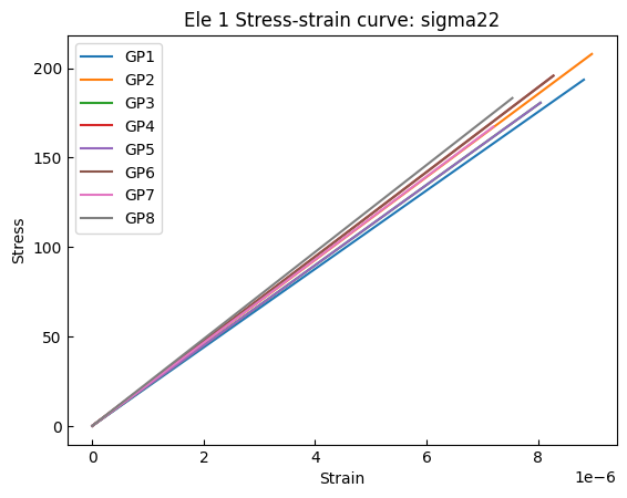
[10]:
stresses2 = stresses.sel(eleTags=1, DOFs="sigma_vm")
strains2 = strains.sel(eleTags=1, DOFs="sigma_vm")
gauss_points = stresses2.coords["GaussPoints"].data
[11]:
for gp_no in gauss_points:
    s = stresses2.sel(GaussPoints=gp_no)
    d = strains2.sel(GaussPoints=gp_no)
    plt.plot(d, s, label=f"GP{gp_no}")
plt.title("Ele 1 Stress-strain curve: sigma22")
plt.xlabel("Strain")
plt.ylabel("Stress")
plt.legend()
plt.show()
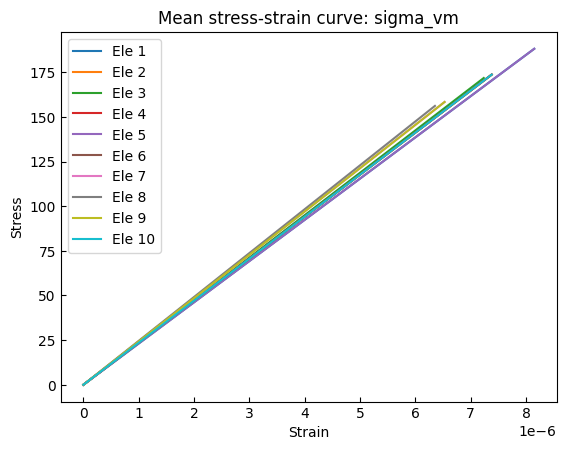
We can also compute averages along a specific dimension. For example, below, we calculate the average stress at the Gauss points:
[12]:
stresses2 = stresses.sel(DOFs="sigma_vm")
strains2 = strains.sel(DOFs="sigma_vm")
stresses3 = stresses2.mean(dim="GaussPoints")
strains3 = strains2.mean(dim="GaussPoints")
[13]:
for eletag in np.arange(1, 11):
    s = stresses3.sel(eleTags=eletag)
    d = strains3.sel(eleTags=eletag)
    plt.plot(d, s, label=f"Ele {eletag}")
plt.title("Mean stress-strain curve: sigma_vm")
plt.xlabel("Strain")
plt.ylabel("Stress")
plt.legend()
plt.show()