✅Fiber Section Visualization

classes GetFEMdata and plot_fiber_sec(), FiberSecVis are needed.

import numpy as np
import openseespy.opensees as ops
import opstool as opst

OpenSeesPy Model Creation

Here we create a pier example.

ops.wipe()
ops.model('basic', '-ndm', 3, '-ndf', 6)

def create_pier(sec_tag):
    ops.node(1, 0.0, 0.0, 0.0)
    ops.node(2, 0.0, 0.0, 6.0)
    ops.mass(2, 50, 50, 50, 0.0, 0.0, 0.0)
    ops.fix(1, 1, 1, 1, 1, 1, 1)
    ops.geomTransf('Linear', 1, *[-1.0, 0.0, 0.0])
    ops.beamIntegration('Lobatto', 1, sec_tag, 6)
    ops.element('forceBeamColumn', 1, *[1, 2], 1, 1)

Next we use opstool.preprocessing.SecMesh to create a fiber section, or define it yourself.

outlines = [[0, 0], [1, 0], [1, 1], [0, 1]]
coverlines = opst.offset(outlines, d=0.05)
cover = opst.add_polygon(outlines, holes=[coverlines])
holelines = [[0.25, 0.25], [0.75, 0.25], [0.75, 0.75], [0.25, 0.75]]
core = opst.add_polygon(coverlines, holes=[holelines])
# ------------------------------------------------------------
sec = opst.SecMesh()
sec.assign_group(dict(cover=cover, core=core))
sec.assign_mesh_size(dict(cover=0.001, core=0.005))
sec.assign_group_color(dict(cover="gray", core="green"))
# Specify the material tag in the opensees, the material needs to be defined by you beforehand.
ops.uniaxialMaterial('Concrete01', 1, -25.E3, -0.002, -10.E3, -0.005)
ops.uniaxialMaterial('Concrete01', 2, -40.E3, -0.006, -30.E3, -0.015)
sec.assign_ops_matTag(dict(cover=1, core=2))
sec.mesh()
# ------------------------------------------------------------
# add rebars
ops.uniaxialMaterial('Steel01', 3, 200.E3, 2.E8, 0.02)
rebars = opst.Rebars()
rebar_lines1 = opst.offset(outlines, d=0.05 + 0.032 / 2)
rebars.add_rebar_line(
    points=rebar_lines1, dia=0.032, gap=0.1, color="red", matTag=3
)
rebar_lines2 = opst.offset(holelines, d=-(0.05 + 0.02 / 2))
rebars.add_rebar_line(
    points=rebar_lines2, dia=0.020, gap=0.1, color="black", matTag=3
)
# add to the sec
sec.add_rebars(rebars)
# -----------------------------------------------------------------------------
sec.centring()
sec.view(fill=True, engine='plotly', save_html=None, on_notebook=True)

sec_props = sec.get_frame_props(display_results=True)
G = 3.45E7 / (2 * (1 + 0.2))
J = sec_props['J']  # or other number if you don't care
sec.opspy_cmds(secTag=1, GJ=G * J)   # generate openseespy fiber commands

                           Frame Section Properties                            
┏━━━━━━━━━━━┳━━━━━━━━━━━━━━━━━━━━━━━━┳━━━━━━━━━━━━━━━━━━━━━━━━━━━━━━━━━━━━━━━━┓
┃ Symbol    ┃ Value                  ┃ Definition                             ┃
┡━━━━━━━━━━━╇━━━━━━━━━━━━━━━━━━━━━━━━╇━━━━━━━━━━━━━━━━━━━━━━━━━━━━━━━━━━━━━━━━┩
│ A         │ 7.500E-01              │ Cross-sectional area                   │
│ centroid  │ (5.000E-01, 5.000E-01) │ Elastic centroid                       │
│ Iy        │ 7.813E-02              │ Moment of inertia y-axis               │
│ Iz        │ 7.813E-02              │ Moment of inertia z-axis               │
│ Iyz       │ 4.441E-16              │ Product of inertia                     │
│ Wyt       │ 1.564E+14              │ Section moduli of top fibres y-axis    │
│ Wyb       │ 7.813E-02              │ Section moduli of bottom fibres y-axis │
│ Wzt       │ 6.702E+13              │ Section moduli of top fibres z-axis    │
│ Wzb       │ 7.813E-02              │ Section moduli of bottom fibres z-axis │
│ J         │ -2.457E-01             │ Torsion constant                       │
│ phi       │ 0.000E+00              │ Principal axis angle                   │
│ mass      │ 7.500E-01              │ Section mass                           │
│ rho_rebar │ 4.586E-02              │ Ratio of reinforcement                 │
└───────────┴────────────────────────┴────────────────────────────────────────┘

create_pier(sec_tag=1)

Visualization of fiber section geometry information

Get the fiber section data, note that for parameter ele_sec you should enter a list where each item is a element-section pair, e.g. [(1,1),(1,2), (2,1), ….] , i.e. element 1 and 1# integral point section, element 1 and 2# integral point section, etc.

Method get_fiber_data() will save all fiber data in ele_sec.

Since this is a single pier model with one element and 6 intergration points, we can set [(1,1), (1, 2), (1, 3)] and so on.

ele_sec = []
for i in range(6):
    ele_sec.append((1, i+1))

FEMdata = opst.GetFEMdata()
FEMdata.get_fiber_data(ele_sec=ele_sec, save_file='FiberData.hdf5')

Fiber section data saved in opstool_output/FiberData.hdf5!

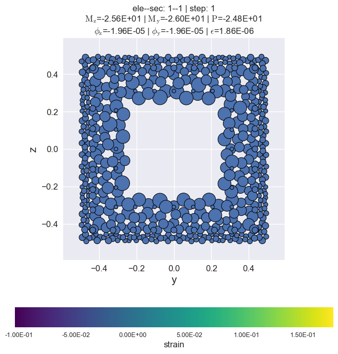
Visualization of fiber cross-sections by plot_fiber_sec(). Since only the location and area information of the fiber points can be extracted, a series of circles is used for rendering.

opst.plot_fiber_sec(ele_sec=[(1,1)],
                   results_dir="opstool_output",
                   input_file='FiberData.hdf5')

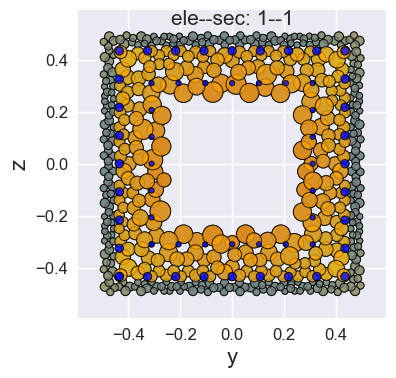
Of course, you can also use a custom color dict, where the keys are the OpenSeesPy material tags in the cross section and the values are any matplotlib supported color labels.

opst.plot_fiber_sec(ele_sec=[(1,1)],
                   results_dir="opstool_output",
                   input_file='FiberData.hdf5',
                   mat_color={1: 'gray', 2: 'orange', 3: 'blue'})

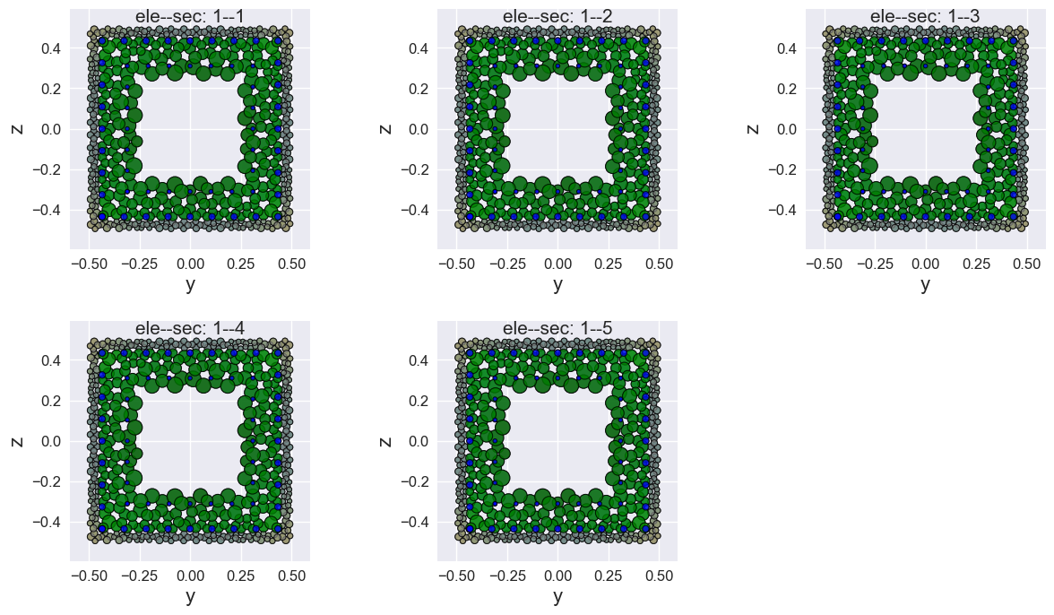
You can also draw multiple fiber sections at once, if you have different sections.

opst.plot_fiber_sec(ele_sec=ele_sec[:-1],
                   results_dir="opstool_output",
                   input_file='FiberData.hdf5',
                   mat_color={1: 'gray', 2: 'green', 3: 'blue'})

Fiber section responses visualization

applying the dynamic load

# --------------------------------------------------
# dynamic load
ops.rayleigh(0.0, 0.0, 0.0, 0.000625)
ops.loadConst('-time', 0.0)

# applying Dynamic Ground motion analysis
dt = 0.02
ttot = 5
npts = int(ttot / dt)
x = np.linspace(0, ttot, npts)
data = 2.0 * np.sin(2 * np.pi * x)
ops.timeSeries('Path', 2, '-dt', dt, '-values', *data, '-factor', 9.81)
ops.pattern('UniformExcitation', 2, 1, '-accel', 2)
ops.pattern('UniformExcitation', 3, 2, '-accel', 2)

ops.wipeAnalysis()
ops.system('BandGeneral')
# Create the constraint handler, the transformation method
ops.constraints('Transformation')
# Create the DOF numberer, the reverse Cuthill-McKee algorithm
ops.numberer('RCM')
ops.test('NormDispIncr', 1e-8, 10)
ops.algorithm('Linear')
ops.integrator('Newmark', 0.5, 0.25)
ops.analysis('Transient')

Get the response data for each analysis step.

Note

get_resp_step() can be used to get all responses type data. save_resp_all() will save data after loop.

for i in range(npts):
    ops.analyze(1, dt)
    FEMdata.get_resp_step()
# save all responses data after loop
FEMdata.save_resp_all(save_file="RespStepData-1.hdf5")

Model data saved in opstool_output/ModelData.hdf5!

All responses data saved in opstool_output/RespStepData-1.hdf5!

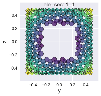
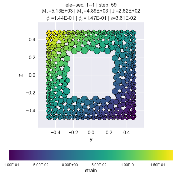
Visualization of the maximum response step if step is None.

resp_vis() can accept the show_variable as “stress” or “strain”. show_mats can be set if you only want to display the response of some materials, the elements must be the material tags that have been defined in the previous opensees commands, and must be included in this section.

secvis = opst.FiberSecVis(input_file="RespStepData-1.hdf5", opacity=1, colormap='viridis')
secvis.resp_vis(ele_tag=1, sec_tag=1,
                step=None,
                show_variable='strain',
                show_mats=[1, 2, 3],)

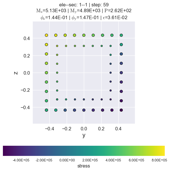
stress of rebars by matTag 3

secvis.resp_vis(ele_tag=1, sec_tag=1,
                step=None,
                show_variable='stress',
                show_mats=[3],)

Generate animated gif files.

secvis.animation(ele_tag=1, sec_tag=1,
                 output_file='images/sec1-1.gif',
                 show_variable='strain',
                 show_mats=[1, 2, 3],
                 framerate=10)

MovieWriter ffmpeg unavailable; using Pillow instead.

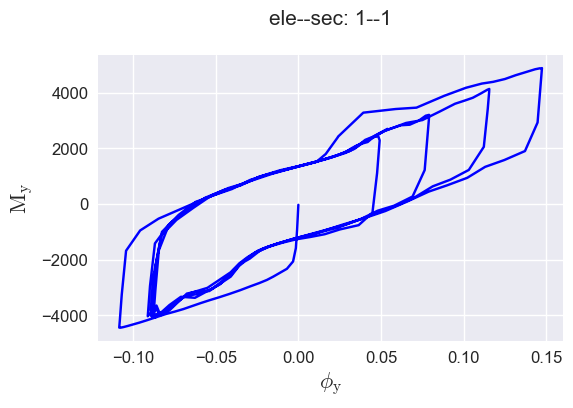
plot forces-deformations relationship

defos, forces = secvis.force_defo_vis(ele_tag=1, sec_tag=1,
                                      force_type="My",
                                      defo_type="Phiy")