Moment Curvature Analysis of Section
[1]:
import opstool as opst
import openseespy.opensees as ops
import matplotlib.pyplot as plt
Create Section
Note
This step is not mandatory. You can also use your own section, as the subsequent analysis only requires the section tag.
Note that you need to set the model to 6DOF in 3D, because the program takes two axes into account.
Create any opensees material yourself as follows:
[2]:
def create_section():
    ops.wipe()
    ops.model("basic", "-ndm", 3, "-ndf", 6)
    # materials
    Ec = 3.55e7
    Vc = 0.2
    Gc = 0.5 * Ec / (1 + Vc)
    fc = -32.4e3
    ec = -2000.0e-6
    ecu = 2.1 * ec
    ft = 2.64e3
    et = 107e-6
    fccore = -40.6e3
    eccore = -4079e-6
    ecucore = -0.0144
    Fys = 300.0e3
    Es = 2.0e8
    bs = 0.01
    matTagC = 1
    matTagCCore = 2
    matTagS = 3
    # for cover
    ops.uniaxialMaterial("Concrete04", matTagC, fc, ec, ecu, Ec, ft, et)
    # for core
    ops.uniaxialMaterial("Concrete04", matTagCCore, fccore, eccore, ecucore, Ec, ft, et)
    ops.uniaxialMaterial(
        "Steel01",
        matTagS,
        Fys,
        Es,
        bs,
    )
    outlines = [[0, 0], [2, 0], [2, 2], [0, 2]]
    coverlines = opst.pre.section.offset(outlines, d=0.05)
    cover = opst.pre.section.create_polygon_patch(outlines, holes=[coverlines])
    holelines = [[0.5, 0.5], [1.5, 0.5], [1.5, 1.5], [0.5, 1.5]]
    core = opst.pre.section.create_polygon_patch(coverlines, holes=[holelines])
    SEC = opst.pre.section.FiberSecMesh()
    SEC.add_patch_group(dict(cover=cover, core=core))
    SEC.set_mesh_size(dict(cover=0.1, core=0.1))
    SEC.set_mesh_color(dict(cover="gray", core="green"))
    SEC.set_ops_mat_tag(dict(cover=matTagC, core=matTagCCore))
    SEC.mesh()
    # add rebars
    rebar_lines = opst.pre.section.offset(outlines, d=0.05 + 0.032 / 2)
    SEC.add_rebar_line(
        points=rebar_lines,
        dia=0.02,
        gap=0.1,
        color="red",
        ops_mat_tag=matTagS,
    )
    SEC.get_frame_props(display_results=False)
    SEC.centring()
    # sec.rotate(45)
    return SEC
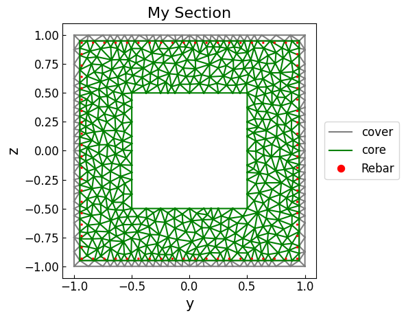
Create the section mesh, see opstool.pre.section.FiberSecMesh
Plot the section mesh:
[3]:
SEC = create_section()
SEC.view(fill=False)
OPSTOOL :: The section My Section has been successfully meshed!
Generate the OpenSeesPy commands to the domin (important!)
[4]:
sec_tag = 1
SEC.to_opspy_cmds(secTag=sec_tag, GJ=100000)
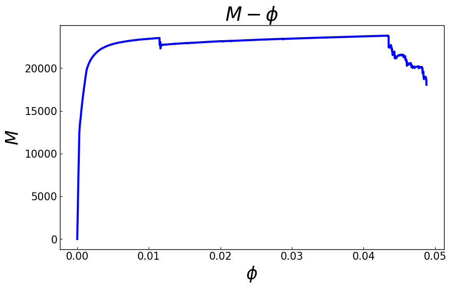
Monotonically Moment-Curvature Analysis
Now you can perform a moment-curvature analysis:
[5]:
MC = opst.anlys.MomentCurvature(sec_tag=1, axial_force=-20000)
MC.analyze(axis="y", max_phi=0.1, incr_phi=1e-5, limit_peak_ratio=0.8, smart_analyze=True)
MomentCurvature: 🎉 Successfully finished! 🎉
Plot the moment-curvature relationship:
[6]:
MC.plot_M_phi()
plt.show()
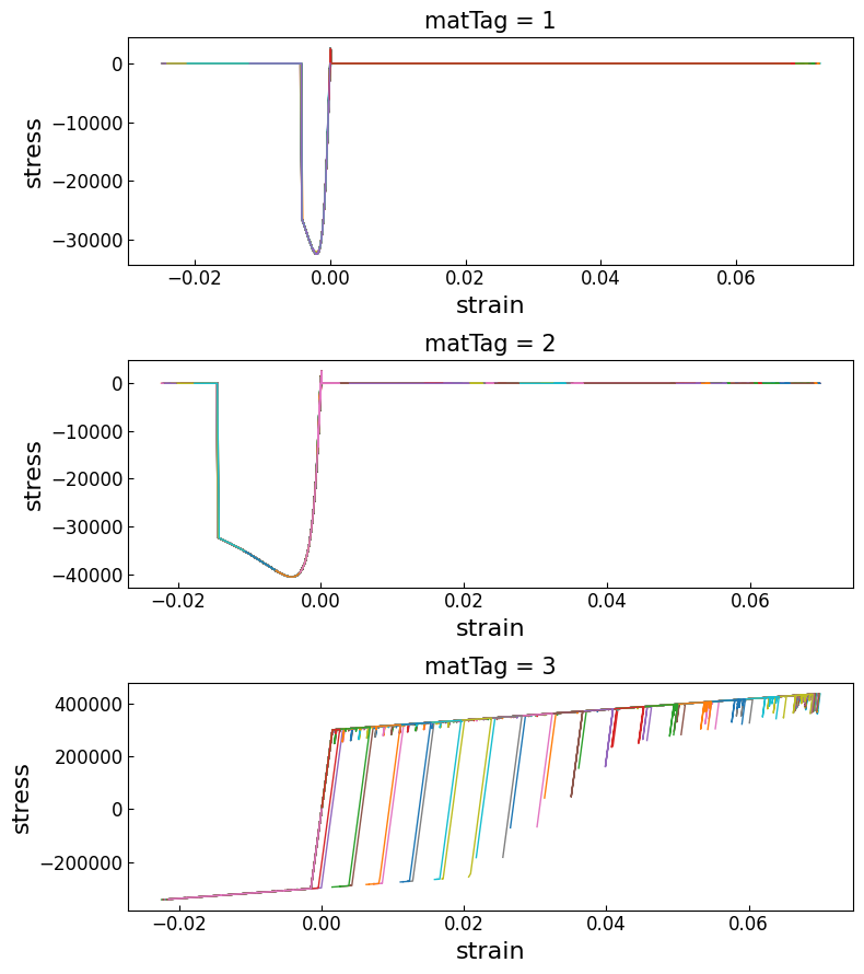
Plot all fiber stress-strain responses:
[7]:
MC.plot_fiber_responses()
plt.show()
[8]:
# Get moment-curvature data
phi, M = MC.get_M_phi()
# Get fiber responses data
fiber_data = MC.get_fiber_data()
fiber_data is an xarray.DataArray structure. "Steps" is the number of steps in the analysis. "Fibers" is the number of fibers in the section. "Properties" is the properties of the fibers, including “yloc”, “zloc”, “area”, “mat”, “stress”, “strain”.
[9]:
print("Fiber data:", fiber_data)
Fiber data: <xarray.DataArray 'FiberData' (Steps: 4881, Fibers: 1199, Properties: 6)> Size: 281MB
array([[[-0.00000000e+00,  0.00000000e+00,  0.00000000e+00,
          0.00000000e+00, -0.00000000e+00, -0.00000000e+00],
        [-0.00000000e+00, -0.00000000e+00,  0.00000000e+00,
          0.00000000e+00, -0.00000000e+00, -0.00000000e+00],
        [ 0.00000000e+00,  0.00000000e+00,  0.00000000e+00,
          0.00000000e+00, -0.00000000e+00, -0.00000000e+00],
        ...,
        [-0.00000000e+00, -0.00000000e+00,  0.00000000e+00,
          0.00000000e+00, -0.00000000e+00, -0.00000000e+00],
        [-0.00000000e+00, -0.00000000e+00,  0.00000000e+00,
          0.00000000e+00, -0.00000000e+00, -0.00000000e+00],
        [-0.00000000e+00, -0.00000000e+00,  0.00000000e+00,
          0.00000000e+00, -0.00000000e+00, -0.00000000e+00]],

       [[-9.66666667e-01,  8.62500000e-01,  1.56250000e-03,
          1.00000000e+00, -6.17687075e+03, -1.76726094e-04],
        [-4.09375000e-01, -9.83333333e-01,  1.56250000e-03,
          1.00000000e+00, -6.80803791e+03, -1.94930340e-04],
        [ 8.62500000e-01,  9.66666667e-01,  1.56250000e-03,
          1.00000000e+00, -6.15403466e+03, -1.76099097e-04],
...
        [-7.37368421e-01, -9.34000000e-01,  3.14159265e-04,
          3.00000000e+00, -3.40004046e+05, -2.15020229e-02],
        [-8.35684211e-01, -9.34000000e-01,  3.14159265e-04,
          3.00000000e+00, -3.39916290e+05, -2.14581451e-02],
        [-9.34000000e-01, -9.34000000e-01,  3.14159265e-04,
          3.00000000e+00, -3.39828535e+05, -2.14142673e-02]],

       [[-9.66666667e-01,  8.62500000e-01,  1.56250000e-03,
          1.00000000e+00,  0.00000000e+00,  6.62158801e-02],
        [-4.09375000e-01, -9.83333333e-01,  1.56250000e-03,
          1.00000000e+00,  0.00000000e+00, -2.41744480e-02],
        [ 8.62500000e-01,  9.66666667e-01,  1.56250000e-03,
          1.00000000e+00,  0.00000000e+00,  7.02684516e-02],
        ...,
        [-7.37368421e-01, -9.34000000e-01,  3.14159265e-04,
          3.00000000e+00, -3.40164332e+05, -2.15821661e-02],
        [-8.35684211e-01, -9.34000000e-01,  3.14159265e-04,
          3.00000000e+00, -3.40053530e+05, -2.15267649e-02],
        [-9.34000000e-01, -9.34000000e-01,  3.14159265e-04,
          3.00000000e+00, -3.39942727e+05, -2.14713637e-02]]])
Coordinates:
  * Steps       (Steps) int32 20kB 0 1 2 3 4 5 ... 4875 4876 4877 4878 4879 4880
  * Fibers      (Fibers) int32 5kB 0 1 2 3 4 5 ... 1193 1194 1195 1196 1197 1198
  * Properties  (Properties) <U6 144B 'yloc' 'zloc' 'area' ... 'stress' 'strain'
[10]:
fiber_data_last = fiber_data.isel(Steps=-1)
y = fiber_data_last.sel(Properties="yloc")
z = fiber_data_last.sel(Properties="zloc")
matTag = fiber_data_last.sel(Properties="mat")
stress = fiber_data_last.sel(Properties="stress")
strain = fiber_data_last.sel(Properties="strain")
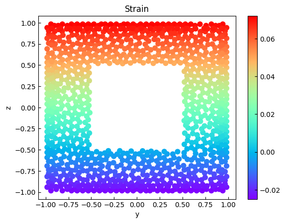
[11]:
plt.figure()
s = plt.scatter(y, z, c=strain, s=50, cmap="rainbow")
plt.colorbar(s)
plt.xlabel("y")
plt.ylabel("z")
plt.title("Strain")
plt.show()
Extract limit state points based on fiber strain thresholds or other criteria.
[12]:
# Tensile steel fibers yield (strain=2e-3) for the first time
phiy, My = MC.get_limit_state(
    matTag=3,  # Steel material tag
    threshold=2e-3,
)
# The concrete fiber in the confined area reaches the ultimate compressive strain 0.0144
phiu, Mu = MC.get_limit_state(matTag=2, threshold=-0.0144, peak_drop=False)
# or use peak_drop
# phiu, Mu = mc.get_limit_state(matTag=2,
#                               threshold=-0.0144,
#                               peak_drop=0.2
#                              )

print(f"Limit state 1: phi_y={phiy:.4f}, My={My:.2f}")
print(f"Limit state 2: phi_u={phiu:.4f}, Mu={Mu:.2f}")
Limit state 1: phi_y=0.0016, My=20552.69
Limit state 2: phi_u=0.0434, Mu=23749.61
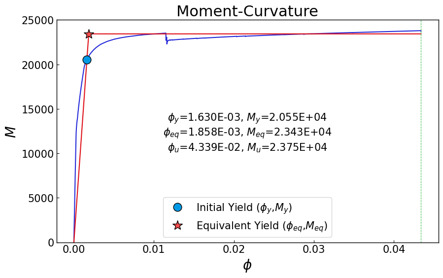
Equivalent linearization according to area:
[13]:
phi_eq, M_eq = MC.bilinearize(phiy, My, phiu, plot=True)
plt.show()
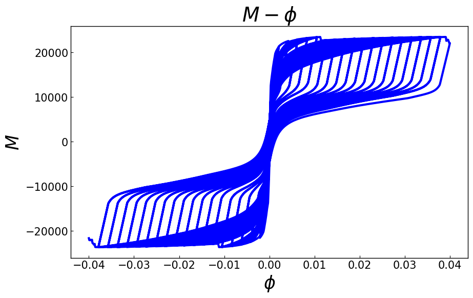
Cycle Moment-Curvature Analysis
[14]:
SEC = create_section()
sec_tag = 1
SEC.to_opspy_cmds(secTag=sec_tag, GJ=100000)
OPSTOOL :: The section My Section has been successfully meshed!
[15]:
MC = opst.anlys.MomentCurvature(sec_tag=1, axial_force=-20000)
MC.set_cycle_path(max_phi=0.04, n_cycle=20, n_hold=2)
MC.analyze(
    axis="y",
    cycle_analyze=True,
    incr_phi=1e-4,
    limit_peak_ratio=0.8,
    smart_analyze=True,
)
MomentCurvature: 🎉 Successfully finished! 🎉
[16]:
MC.plot_M_phi()
plt.show()