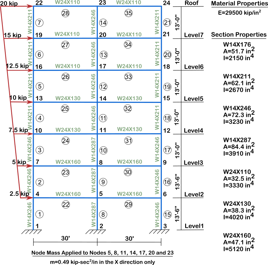
Two-Dimensional Moment Frame Analysis
This is a complete example of frame analysis. Although it is a 2D case, it can be applied to more complex models. While it demonstrates linear elastic analysis, it is also applicable to nonlinear elastoplastic analysis.
[7]:
import numpy as np
import openseespy.opensees as ops
import opstool as opst
import opstool.vis.pyvista as opsvis
import matplotlib.pyplot as plt
import matplotlib.ticker as ticker
Create the model
[8]:
def FEModel():
ops.wipe()
ops.model("basic", "-ndm", 2, "-ndf", 3)
# %% Defining Nodes
ops.node(1, 0.000000e00, 0.000000e00)
ops.node(2, 3.600000e02, 0.000000e00)
ops.node(3, 7.200000e02, 0.000000e00)
ops.node(4, 0.000000e00, 1.620000e02)
ops.node(5, 3.600000e02, 1.620000e02)
ops.node(6, 7.200000e02, 1.620000e02)
ops.node(7, 0.000000e00, 3.240000e02)
ops.node(8, 3.600000e02, 3.240000e02)
ops.node(9, 7.200000e02, 3.240000e02)
ops.node(10, 0.000000e00, 4.800000e02)
ops.node(11, 3.600000e02, 4.800000e02)
ops.node(12, 7.200000e02, 4.800000e02)
ops.node(13, 0.000000e00, 6.360000e02)
ops.node(14, 3.600000e02, 6.360000e02)
ops.node(15, 7.200000e02, 6.360000e02)
ops.node(16, 0.000000e00, 7.920000e02)
ops.node(17, 3.600000e02, 7.920000e02)
ops.node(18, 7.200000e02, 7.920000e02)
ops.node(19, 0.000000e00, 9.480000e02)
ops.node(20, 3.600000e02, 9.480000e02)
ops.node(21, 7.200000e02, 9.480000e02)
ops.node(22, 0.000000e00, 1.104000e03)
ops.node(23, 3.600000e02, 1.104000e03)
ops.node(24, 7.200000e02, 1.104000e03)
# %% write node restraint
ops.fix(1, 1, 1, 1)
ops.fix(2, 1, 1, 1)
ops.fix(3, 1, 1, 1)
# %% Define the rigidDiaphragm
ops.rigidDiaphragm(1, 5, 4, 6)
ops.rigidDiaphragm(1, 8, 7, 9)
ops.rigidDiaphragm(1, 11, 10, 12)
ops.rigidDiaphragm(1, 14, 13, 15)
ops.rigidDiaphragm(1, 17, 16, 18)
ops.rigidDiaphragm(1, 20, 19, 21)
ops.rigidDiaphragm(1, 23, 22, 24)
# %% Defining Frame Elements
ops.geomTransf("Linear", 1)
ops.element("elasticBeamColumn", 1, 1, 4, 7.230000e01, 2.950000e04,
3.230000e03, 1)
ops.element("elasticBeamColumn", 2, 4, 7, 7.230000e01, 2.950000e04,
3.230000e03, 1)
ops.element("elasticBeamColumn", 3, 7, 10, 7.230000e01, 2.950000e04,
3.230000e03, 1)
ops.element("elasticBeamColumn", 4, 10, 13, 6.210000e01, 2.950000e04,
2.670000e03, 1)
ops.element("elasticBeamColumn", 5, 13, 16, 6.210000e01, 2.950000e04,
2.670000e03, 1)
ops.element("elasticBeamColumn", 6, 16, 19, 5.170000e01, 2.950000e04,
2.150000e03, 1)
ops.element("elasticBeamColumn", 7, 19, 22, 5.170000e01, 2.950000e04,
2.150000e03, 1)
ops.element("elasticBeamColumn", 8, 2, 5, 8.440000e01, 2.950000e04,
3.910000e03, 1)
ops.element("elasticBeamColumn", 9, 5, 8, 8.440000e01, 2.950000e04,
3.910000e03, 1)
ops.element("elasticBeamColumn", 10, 8, 11, 8.440000e01, 2.950000e04,
3.910000e03, 1)
ops.element("elasticBeamColumn", 11, 11, 14, 7.230000e01, 2.950000e04,
3.230000e03, 1)
ops.element("elasticBeamColumn", 12, 14, 17, 7.230000e01, 2.950000e04,
3.230000e03, 1)
ops.element("elasticBeamColumn", 13, 17, 20, 6.210000e01, 2.950000e04,
2.670000e03, 1)
ops.element("elasticBeamColumn", 14, 20, 23, 6.210000e01, 2.950000e04,
2.670000e03, 1)
ops.element("elasticBeamColumn", 15, 3, 6, 7.230000e01, 2.950000e04,
3.230000e03, 1)
ops.element("elasticBeamColumn", 16, 6, 9, 7.230000e01, 2.950000e04,
3.230000e03, 1)
ops.element("elasticBeamColumn", 17, 9, 12, 7.230000e01, 2.950000e04,
3.230000e03, 1)
ops.element("elasticBeamColumn", 18, 12, 15, 6.210000e01, 2.950000e04,
2.670000e03, 1)
ops.element("elasticBeamColumn", 19, 15, 18, 6.210000e01, 2.950000e04,
2.670000e03, 1)
ops.element("elasticBeamColumn", 20, 18, 21, 5.170000e01, 2.950000e04,
2.150000e03, 1)
ops.element("elasticBeamColumn", 21, 21, 24, 5.170000e01, 2.950000e04,
2.150000e03, 1)
ops.element("elasticBeamColumn", 22, 4, 5, 4.710000e01, 2.950000e04,
5.120000e03, 1)
ops.element("elasticBeamColumn", 23, 7, 8, 4.710000e01, 2.950000e04,
5.120000e03, 1)
ops.element("elasticBeamColumn", 24, 10, 11, 3.830000e01, 2.950000e04,
4.020000e03, 1)
ops.element("elasticBeamColumn", 25, 13, 14, 3.830000e01, 2.950000e04,
4.020000e03, 1)
ops.element("elasticBeamColumn", 26, 16, 17, 3.250000e01, 2.950000e04,
3.330000e03, 1)
ops.element("elasticBeamColumn", 27, 19, 20, 3.250000e01, 2.950000e04,
3.330000e03, 1)
ops.element("elasticBeamColumn", 28, 22, 23, 3.250000e01, 2.950000e04,
3.330000e03, 1)
ops.element("elasticBeamColumn", 29, 5, 6, 4.710000e01, 2.950000e04,
5.120000e03, 1)
ops.element("elasticBeamColumn", 30, 8, 9, 4.710000e01, 2.950000e04,
5.120000e03, 1)
ops.element("elasticBeamColumn", 31, 11, 12, 3.830000e01, 2.950000e04,
4.020000e03, 1)
ops.element("elasticBeamColumn", 32, 14, 15, 3.830000e01, 2.950000e04,
4.020000e03, 1)
ops.element("elasticBeamColumn", 33, 17, 18, 3.250000e01, 2.950000e04,
3.330000e03, 1)
ops.element("elasticBeamColumn", 34, 20, 21, 3.250000e01, 2.950000e04,
3.330000e03, 1)
ops.element("elasticBeamColumn", 35, 23, 24, 3.250000e01, 2.950000e04,
3.330000e03, 1)
# %% Define the mass
ops.mass(5, 0.49, 0.0, 0.0)
ops.mass(8, 0.49, 0.0, 0.0)
ops.mass(11, 0.49, 0.0, 0.0)
ops.mass(14, 0.49, 0.0, 0.0)
ops.mass(17, 0.49, 0.0, 0.0)
ops.mass(20, 0.49, 0.0, 0.0)
ops.mass(23, 0.49, 0.0, 0.0)
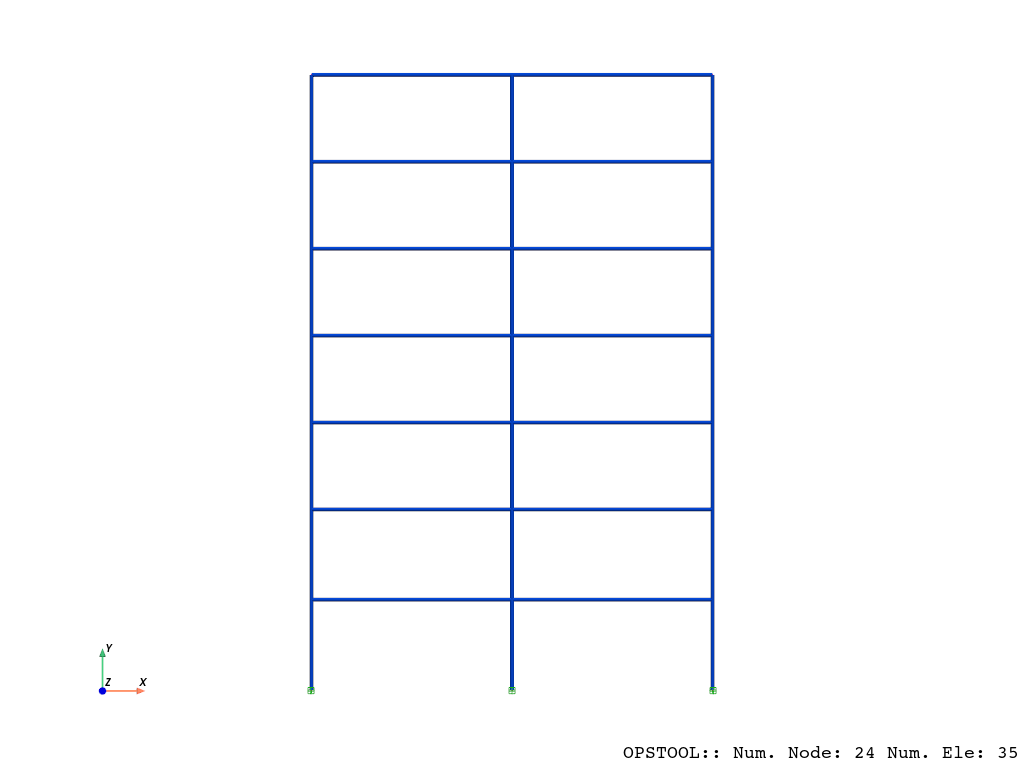
Let’s first visualize the geometry:
[9]:
FEModel()
# If you work on notebook, you can use the following code to visualize the model
opsvis.set_plot_props(line_width=4, point_size=2, notebook=True)
opsvis.plot_model().show(jupyter_backend="jupyterlab") # For static plot
# opsvis.plot_model().show() # For interactive plot
# If you work on script, you can use the following code to visualize the model
# opsvis.set_plot_props(line_width=4, point_size=2)
# opsvis.plot_model().show()
OPSTOOL :: Model data has been saved to _OPSTOOL_ODB/ModelData-None.nc!
You can also use the following code to visualize the model by using Plotly:
[10]:
opst.vis.plotly.set_plot_props(line_width=4, point_size=2)
fig = opst.vis.plotly.plot_model()
fig.write_html("model.html")
fig.show()
OPSTOOL :: Model data has been saved to _OPSTOOL_ODB/ModelData-None.nc!
Data type cannot be displayed: application/vnd.plotly.v1+json
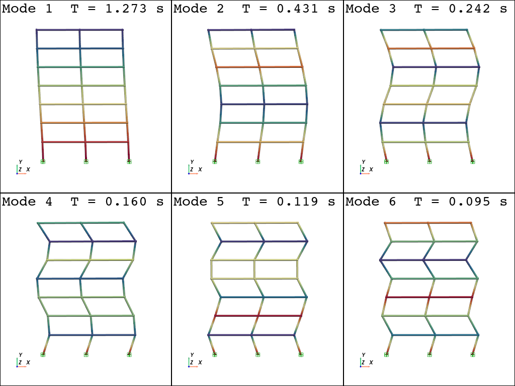
Eigenvalue analysis
solver=”-fullGenLapack” is intended to extract all seventh-order modes. This solver should be avoided in actual large models.
[11]:
opst.post.save_eigen_data(odb_tag="eigen", mode_tag=7, solver="-fullGenLapack")
opsvis.set_plot_props(cmap="Spectral",
line_width=4,
point_size=5,
font_size=12,
notebook=True)
WARNING - the 'fullGenLapack' eigen solver is VERY SLOW. Consider using the default eigen solver.Using DomainModalProperties - Developed by: Massimo Petracca, Guido Camata, ASDEA Software Technology
OPSTOOL :: Eigen data has been saved to _OPSTOOL_ODB/EigenData-eigen.nc!
[12]:
opsvis.plot_eigen(
mode_tags=[1, 6],
odb_tag="eigen",
subplots=True,
bc_scale=3,
).show(jupyter_backend="jupyterlab")
OPSTOOL :: Loading eigen data from _OPSTOOL_ODB/EigenData-eigen.nc ...
[13]:
model_props, eigen_vectors = opst.post.get_eigen_data(odb_tag="eigen")
model_props_df = model_props.to_pandas() # to pandas DataFrame
print("Modal period: ", model_props_df["eigenPeriod"])
print("Participation mass ratio: ", model_props_df["partiMassRatiosMX"])
print("Cumulative participation mass ratio: ",
model_props_df["partiMassRatiosCumuMX"])
OPSTOOL :: Loading eigen data from _OPSTOOL_ODB/EigenData-eigen.nc ...
Modal period: modeTags
1 1.273211
2 0.431278
3 0.242043
4 0.160179
5 0.118990
6 0.095064
7 0.079515
Name: eigenPeriod, dtype: float64
Participation mass ratio: modeTags
1 79.962669
2 11.336182
3 4.180994
4 2.115029
5 1.414555
6 0.679967
7 0.310604
Name: partiMassRatiosMX, dtype: float64
Cumulative participation mass ratio: modeTags
1 79.962669
2 91.298850
3 95.479845
4 97.594874
5 99.009429
6 99.689396
7 100.000000
Name: partiMassRatiosCumuMX, dtype: float64
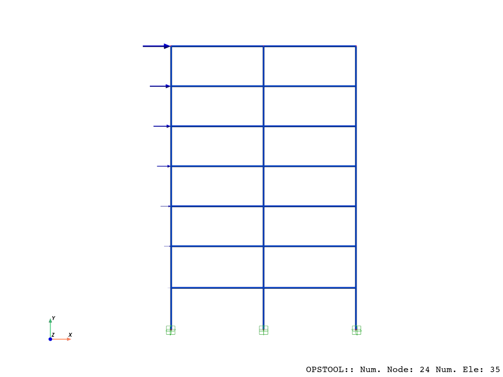
Static analysis
Defining Lateral Distributed Loads:
[14]:
FEModel()
# %% Define the load pattern
ops.timeSeries("Linear", 1)
ops.pattern("Plain", 1, 1)
ops.load(4, 2.5, 0.0, 0.0)
ops.load(7, 5.0, 0.0, 0.0)
ops.load(10, 7.5, 0.0, 0.0)
ops.load(13, 10.0, 0.0, 0.0)
ops.load(16, 12.5, 0.0, 0.0)
ops.load(19, 15.0, 0.0, 0.0)
ops.load(22, 20.0, 0.0, 0.0)
Re-examine the model:
[15]:
opsvis.set_plot_props(line_width=4, point_size=4, font_size=12, notebook=True)
opsvis.plot_model(
show_nodal_loads=True,
load_scale=2,
bc_scale=3,
).show(jupyter_backend="jupyterlab")
OPSTOOL :: Model data has been saved to _OPSTOOL_ODB/ModelData-None.nc!
To perform the analysis:
[16]:
n_steps = 10
ops.system("BandGeneral")
ops.constraints("Transformation")
ops.numberer("RCM")
ops.test("NormDispIncr", 1.0e-12, 10, 3)
ops.algorithm("Linear")
ops.integrator("LoadControl", 1 / n_steps)
ops.analysis("Static")
Save data:
[17]:
odb = opst.post.CreateODB(odb_tag="static")
for i in range(n_steps):
ops.analyze(1) # one step of analysis
odb.fetch_response_step() # fetch the response on the current step
odb.save_response()
OPSTOOL :: All responses data with odb_tag = static saved in _OPSTOOL_ODB/RespStepData-static.nc!
Retrieve the nodal displacements:
[18]:
node_resp = opst.post.get_nodal_responses(odb_tag="static")
print(
"Node 22 displacement in x direction: ",
node_resp["disp"].sel(nodeTags=22, DOFs="UX").data[-1],
)
OPSTOOL :: Loading None response data from _OPSTOOL_ODB/RespStepData-static.nc ...
Node 22 displacement in x direction: 1.4507570054071395
Retrieve element response:
[19]:
ele_resp = opst.post.get_element_responses(odb_tag="static",
ele_type="Frame",
resp_type="sectionForces")
print("M:", ele_resp.sel(eleTags=1, secDofs="MZ", secPoints=1).data[-1])
print("V:", ele_resp.sel(eleTags=1, secDofs="VY", secPoints=1).data[-1])
print("N:", ele_resp.sel(eleTags=1, secDofs="N", secPoints=1).data[-1])
OPSTOOL :: Loading Frame sectionForces response data from _OPSTOOL_ODB/RespStepData-static.nc ...
M: -2324.677292913693
V: 20.672081658070365
N: 69.98673407265717
[20]:
print(ele_resp)
<xarray.DataArray 'sectionForces' (time: 11, eleTags: 35, secPoints: 7,
secDofs: 6)> Size: 129kB
array([[[[-0.00000000e+00, 0.00000000e+00, 0.00000000e+00,
-0.00000000e+00, -0.00000000e+00, -0.00000000e+00],
[-0.00000000e+00, 0.00000000e+00, 0.00000000e+00,
-0.00000000e+00, -0.00000000e+00, -0.00000000e+00],
[-0.00000000e+00, 0.00000000e+00, 0.00000000e+00,
-0.00000000e+00, -0.00000000e+00, -0.00000000e+00],
...,
[-0.00000000e+00, 0.00000000e+00, 0.00000000e+00,
-0.00000000e+00, -0.00000000e+00, -0.00000000e+00],
[-0.00000000e+00, 0.00000000e+00, 0.00000000e+00,
-0.00000000e+00, -0.00000000e+00, -0.00000000e+00],
[-0.00000000e+00, 0.00000000e+00, 0.00000000e+00,
-0.00000000e+00, -0.00000000e+00, -0.00000000e+00]],
[[-0.00000000e+00, 0.00000000e+00, 0.00000000e+00,
-0.00000000e+00, -0.00000000e+00, -0.00000000e+00],
[-0.00000000e+00, 0.00000000e+00, 0.00000000e+00,
-0.00000000e+00, -0.00000000e+00, -0.00000000e+00],
[-0.00000000e+00, 0.00000000e+00, 0.00000000e+00,
-0.00000000e+00, -0.00000000e+00, -0.00000000e+00],
...
[-0.00000000e+00, -3.83566586e+02, -5.88506091e+00,
-0.00000000e+00, -0.00000000e+00, -0.00000000e+00],
[-0.00000000e+00, -7.36670241e+02, -5.88506091e+00,
-0.00000000e+00, -0.00000000e+00, -0.00000000e+00],
[-0.00000000e+00, -1.08977390e+03, -5.88506091e+00,
-0.00000000e+00, -0.00000000e+00, -0.00000000e+00]],
[[-0.00000000e+00, 4.77331642e+02, -2.79187109e+00,
-0.00000000e+00, -0.00000000e+00, -0.00000000e+00],
[-0.00000000e+00, 3.09819377e+02, -2.79187109e+00,
-0.00000000e+00, -0.00000000e+00, -0.00000000e+00],
[-0.00000000e+00, 1.42307112e+02, -2.79187109e+00,
-0.00000000e+00, -0.00000000e+00, -0.00000000e+00],
...,
[-0.00000000e+00, -1.92717419e+02, -2.79187109e+00,
-0.00000000e+00, -0.00000000e+00, -0.00000000e+00],
[-0.00000000e+00, -3.60229684e+02, -2.79187109e+00,
-0.00000000e+00, -0.00000000e+00, -0.00000000e+00],
[-0.00000000e+00, -5.27741949e+02, -2.79187109e+00,
-0.00000000e+00, -0.00000000e+00, -0.00000000e+00]]]])
Coordinates:
* eleTags (eleTags) int32 140B 1 2 3 4 5 6 7 8 ... 28 29 30 31 32 33 34 35
* secPoints (secPoints) int32 28B 1 2 3 4 5 6 7
* secDofs (secDofs) <U2 48B 'N' 'MZ' 'VY' 'MY' 'VZ' 'T'
* time (time) float64 88B 0.0 0.1 0.2 0.3 0.4 0.5 0.6 0.7 0.8 0.9 1.0
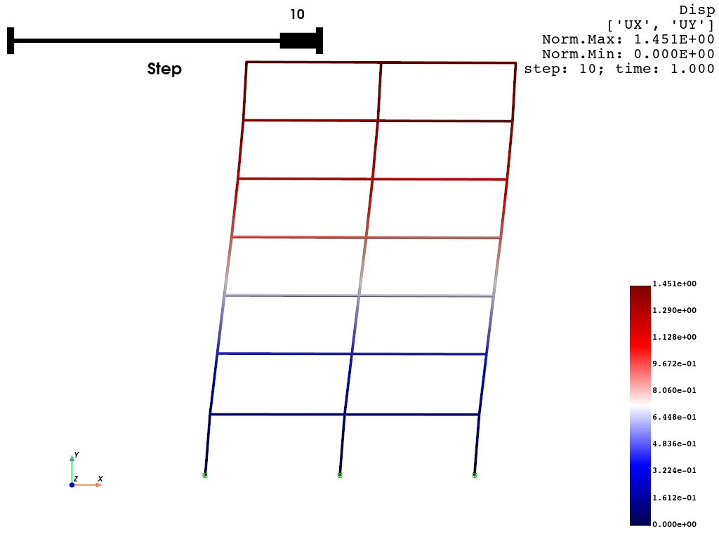
Visualize node responses:
[21]:
opsvis.set_plot_props(cmap="seismic",
notebook=True,
line_width=4,
title_font_size=10)
opsvis.plot_nodal_responses(odb_tag="static",
resp_type="disp",
resp_dof=["UX", "UY"],
slides=True,
scale=2.0).show(jupyter_backend="jupyterlab")
OPSTOOL :: Loading response data from _OPSTOOL_ODB/RespStepData-static.nc ...
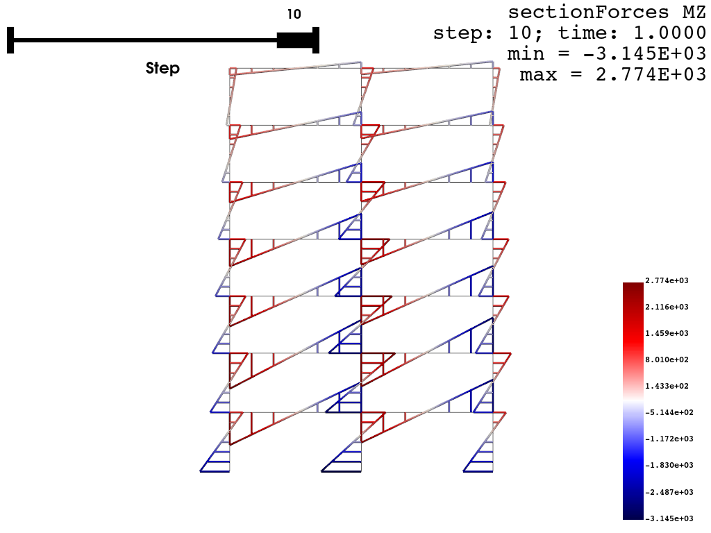
Visualizing Element Response:
[22]:
# Moment response
opsvis.set_plot_props(cmap="seismic",
line_width=1,
notebook=True,
title_font_size=14)
opsvis.plot_frame_responses(
odb_tag="static",
resp_type="sectionForces",
resp_dof="Mz",
slides=True,
scale=-2.0,
line_width=3,
).show(jupyter_backend="jupyterlab")
OPSTOOL :: Loading response data from _OPSTOOL_ODB/RespStepData-static.nc ...
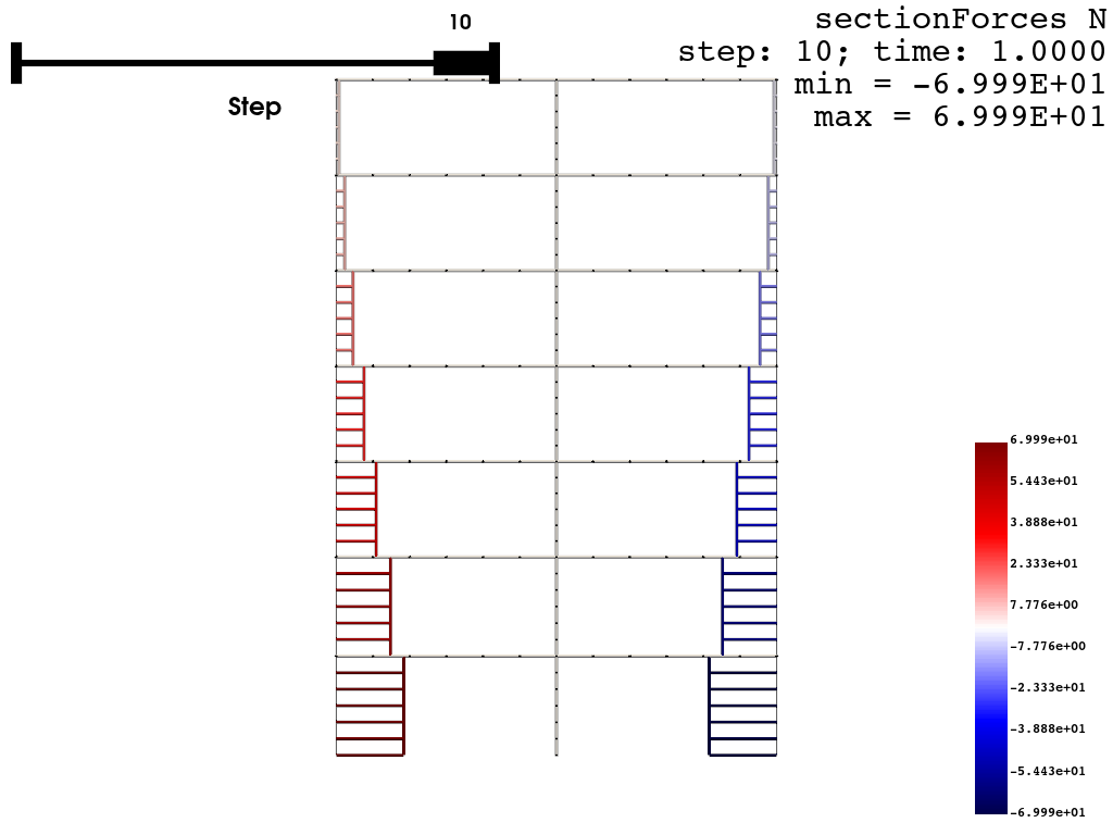
[23]:
# Axial response
opsvis.plot_frame_responses(
odb_tag="static",
resp_type="sectionForces",
resp_dof="N",
slides=True,
scale=-2.0,
line_width=3,
).show(jupyter_backend="jupyterlab")
OPSTOOL :: Loading response data from _OPSTOOL_ODB/RespStepData-static.nc ...
Seismic response analysis
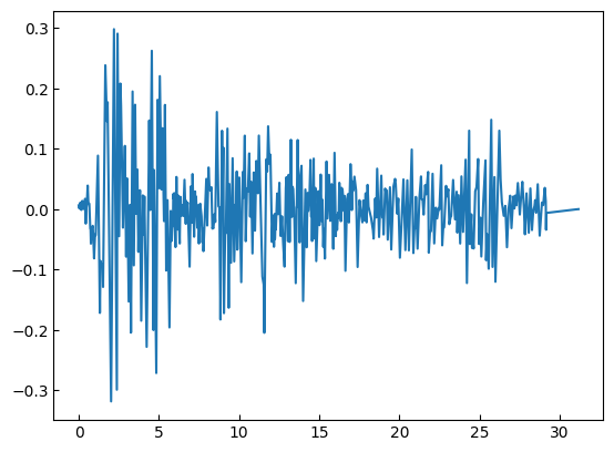
Load the ground motion data
All files can be downloaded here: click
[24]:
gmdata = np.loadtxt("ELCENTRO.txt")
time = gmdata[:, 0]
accel = gmdata[:, 1]
print(len(time))
plt.plot(time, accel)
plt.show()
1560
Create the ground motion load pattern
[25]:
FEModel()
ops.timeSeries("Path", 2, "-time", *time, "-values", *accel, "-factor", 386.4)
ops.pattern("UniformExcitation", 2, 1, "-accel", 2)
Create the Rayleigh damping
[26]:
xDamp = 0.05
MpropSwitch = 1.0
KcurrSwitch = 0.0
KcommSwitch = 1.0
KinitSwitch = 0.0
nEigenI = 1 # mode 1
nEigenJ = 2 # mode 2
lambdaN = ops.eigen(nEigenJ) # eigenvalue analysis for nEigenJ modes
lambdaI = lambdaN[nEigenI - 1] # eigenvalue mode i
lambdaJ = lambdaN[nEigenJ - 1] # eigenvalue mode j
omegaI = np.sqrt(lambdaI)
omegaJ = np.sqrt(lambdaJ)
# M-prop. damping; D = alphaM*M
alphaM = MpropSwitch * xDamp * (2 * omegaI * omegaJ) / (omegaI + omegaJ)
# current-K; +beatKcurr*KCurrent
betaKcurr = KcurrSwitch * 2.0 * xDamp / (omegaI + omegaJ)
# last-committed K; +betaKcomm*KlastCommitt
betaKcomm = KcommSwitch * 2.0 * xDamp / (omegaI + omegaJ)
betaKinit = KinitSwitch * 2.0 * xDamp / (omegaI + omegaJ)
ops.rayleigh(alphaM, 0.0, 0.0, betaKcomm)
Perform analysis and save data
[27]:
ops.wipeAnalysis()
ops.system("BandGeneral")
ops.constraints("Transformation")
ops.numberer("RCM")
ops.test("NormDispIncr", 1.0e-12, 10, 3)
ops.algorithm("Linear")
ops.integrator("HHT", 1.0, 0.5, 0.25)
ops.analysis("Transient")
[28]:
n_steps, dt = 1600, 0.02
odb = opst.post.CreateODB(odb_tag="seismic")
for i in range(n_steps):
ops.analyze(1, dt)
odb.fetch_response_step()
odb.save_response(zlib=True)
# zlib=True to compress the data
OPSTOOL :: All responses data with odb_tag = seismic saved in _OPSTOOL_ODB/RespStepData-seismic.nc!
Retrieve Node Responses
[29]:
node_resp = opst.post.get_nodal_responses(odb_tag="seismic")
node_disp22 = node_resp["disp"].sel(nodeTags=22, DOFs="UX")
node_vel22 = node_resp["vel"].sel(nodeTags=22, DOFs="UX")
node_accel22 = node_resp["accel"].sel(nodeTags=22, DOFs="UX")
OPSTOOL :: Loading None response data from _OPSTOOL_ODB/RespStepData-seismic.nc ...
Read the response result of SAP2000:
[30]:
node_disp22sap = np.loadtxt("output-sap-nodedisp22.txt")
node_vel22sap = np.loadtxt("output-sap-nodevel22.txt")
node_accel22sap = np.loadtxt("output-sap-nodeaccel22.txt")
Draw a time series plot:
[31]:
fig, axes = plt.subplots(3, 1, sharex=True)
time = node_disp22.time
# Define colors and line styles
colors = ["#136ad5", "#fb8a2e"] # Use neutral colors for publication standards
line_styles = ["-", "--"] # Solid and dashed lines for differentiation
# Plot data with clear labels
axes[0].plot(
time,
node_disp22.data,
label="OpenSeesPy+opstool",
color=colors[0],
linestyle=line_styles[0],
linewidth=1.5,
)
axes[0].plot(
time,
node_disp22sap,
label="SAP2000",
color=colors[1],
linestyle=line_styles[1],
linewidth=1.5,
)
axes[1].plot(
time,
node_vel22.data,
label="OpenSeesPy+opstool",
color=colors[0],
linestyle=line_styles[0],
linewidth=1.5,
)
axes[1].plot(
time,
node_vel22sap,
label="SAP2000",
color=colors[1],
linestyle=line_styles[1],
linewidth=1.5,
)
axes[2].plot(
time,
node_accel22.data,
label="OpenSeesPy+opstool",
color=colors[0],
linestyle=line_styles[0],
linewidth=1.5,
)
axes[2].plot(
time,
node_accel22sap,
label="SAP2000",
color=colors[1],
linestyle=line_styles[1],
linewidth=1.5,
)
# Set axis labels and title font sizes
axes[0].set_ylabel("u", fontsize=10)
axes[1].set_ylabel("v", fontsize=10)
axes[2].set_ylabel("a", fontsize=10)
axes[2].set_xlabel("Time (s)", fontsize=10)
# Customize each subplot
for ax in axes:
ax.tick_params(axis="both", which="major",
labelsize=8) # Set tick font size
ax.grid(True, linestyle="--", linewidth=0.5,
alpha=0.7) # Add light grid lines
ax.legend(fontsize=9, loc="best",
frameon=False) # Simple legend without box
# Format X-axis ticks to have consistent significant figures
for ax in axes:
ax.xaxis.set_major_formatter(ticker.FormatStrFormatter("%.1f"))
# Adjust spacing between subplots
fig.subplots_adjust(hspace=0.2) # Adjust vertical spacing
# Save figure in a publication-friendly format
# plt.savefig("fig-node22resp.pdf", bbox_inches="tight")
plt.show()
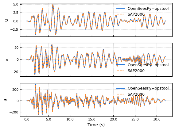
[32]:
print("OpenSees Node 22 Disp Max:", node_disp22.data.max())
print("SAP2000 Node 22 Disp Max:", node_disp22sap.max())
print("OpenSees Node 22 Vel Max:", node_vel22.data.max())
print("SAP2000 Node 22 Vel Max:", node_vel22sap.max())
print("OpenSees Node 22 Accel Max:", node_accel22.data.max())
print("SAP2000 Node 22 Accel Max:", node_accel22sap.max())
print("-" * 50)
print("OpenSees Node 22 Disp Min:", node_disp22.data.min())
print("SAP2000 Node 22 Disp Min:", node_disp22sap.min())
print("OpenSees Node 22 Vel Min:", node_vel22.data.min())
print("SAP2000 Node 22 Vel Min:", node_vel22sap.min())
print("OpenSees Node 22 Accel Min:", node_accel22.data.min())
print("SAP2000 Node 22 Accel Min:", node_accel22sap.min())
OpenSees Node 22 Disp Max: 4.886217886270635
SAP2000 Node 22 Disp Max: 4.886214
OpenSees Node 22 Vel Max: 24.562451885771154
SAP2000 Node 22 Vel Max: 24.56
OpenSees Node 22 Accel Max: 284.12978122981013
SAP2000 Node 22 Accel Max: 284.129
--------------------------------------------------
OpenSees Node 22 Disp Min: -4.141897130769237
SAP2000 Node 22 Disp Min: -4.141893
OpenSees Node 22 Vel Min: -25.27188198677624
SAP2000 Node 22 Vel Min: -25.27
OpenSees Node 22 Accel Min: -249.50410984382438
SAP2000 Node 22 Accel Min: -249.502
Retrieve Element Responses
[33]:
ele_resp = opst.post.get_element_responses(odb_tag="seismic",
ele_type="Frame",
resp_type="sectionForces")
frame1Mz = -ele_resp.sel(eleTags=1, secDofs="MZ", secPoints=1)
frame1N = ele_resp.sel(eleTags=1, secDofs="N", secPoints=1)
frame1Vy = ele_resp.sel(eleTags=1, secDofs="VY", secPoints=1)
OPSTOOL :: Loading Frame sectionForces response data from _OPSTOOL_ODB/RespStepData-seismic.nc ...
[34]:
ele1respSAP = np.loadtxt("output-sap-frame1forces.txt")
frame1NSAP = ele1respSAP[:, 0]
frame1VySAP = ele1respSAP[:, 1]
frame1MzSAP = ele1respSAP[:, 5]
[35]:
fig, axes = plt.subplots(3, 1, sharex=True)
time = frame1Mz.time
# Define colors and line styles
colors = ["#136ad5", "#fb8a2e"] # Use neutral colors for publication standards
line_styles = ["-", "--"] # Solid and dashed lines for differentiation
# Plot data with clear labels
axes[0].plot(
time,
frame1N.data,
label="OpenSeesPy+opstool",
color=colors[0],
linestyle=line_styles[0],
linewidth=1.5,
)
axes[0].plot(
time,
frame1NSAP,
label="SAP2000",
color=colors[1],
linestyle=line_styles[1],
linewidth=1.5,
)
axes[1].plot(
time,
frame1Vy.data,
label="OpenSeesPy+opstool",
color=colors[0],
linestyle=line_styles[0],
linewidth=1.5,
)
axes[1].plot(
time,
frame1VySAP,
label="SAP2000",
color=colors[1],
linestyle=line_styles[1],
linewidth=1.5,
)
axes[2].plot(
time,
frame1Mz.data,
label="OpenSeesPy+opstool",
color=colors[0],
linestyle=line_styles[0],
linewidth=1.5,
)
axes[2].plot(
time,
frame1MzSAP,
label="SAP2000",
color=colors[1],
linestyle=line_styles[1],
linewidth=1.5,
)
# Set axis labels and title font sizes
axes[0].set_ylabel("N", fontsize=10)
axes[1].set_ylabel("V", fontsize=10)
axes[2].set_ylabel("M", fontsize=10)
axes[2].set_xlabel("Time (s)", fontsize=10)
# Customize each subplot
for ax in axes:
ax.tick_params(axis="both", which="major",
labelsize=8) # Set tick font size
ax.grid(True, linestyle="--", linewidth=0.5,
alpha=0.7) # Add light grid lines
ax.legend(fontsize=9, loc="best",
frameon=False) # Simple legend without box
# Format X-axis ticks to have consistent significant figures
for ax in axes:
ax.xaxis.set_major_formatter(ticker.FormatStrFormatter("%.1f"))
# Adjust spacing between subplots
fig.subplots_adjust(hspace=0.2) # Adjust vertical spacing
# Save figure in a publication-friendly format
# plt.savefig("fig-frame1-forces.pdf", bbox_inches="tight")
plt.show()
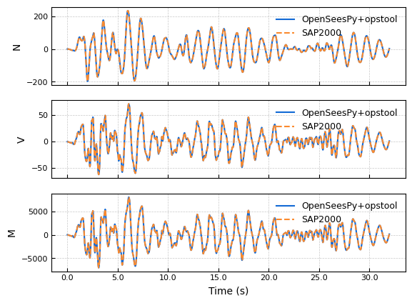
[36]:
print("OpenSees Frame 1 N Max:", frame1N.data.max())
print("SAP2000 Frame 1 N Max:", frame1NSAP.max())
print("OpenSees Frame 1 Vy Max:", frame1Vy.data.max())
print("SAP2000 Frame 1 Vy Max:", frame1VySAP.max())
print("OpenSees Frame 1 Mz Max:", frame1Mz.data.max())
print("SAP2000 Frame 1 Mz Max:", frame1MzSAP.max())
print("-" * 50)
print("OpenSees Frame 1 N Min:", frame1N.data.min())
print("SAP2000 Frame 1 N Min:", frame1NSAP.min())
print("OpenSees Frame 1 Vy Min:", frame1Vy.data.min())
print("SAP2000 Frame 1 Vy Min:", frame1VySAP.min())
print("OpenSees Frame 1 Mz Min:", frame1Mz.data.min())
print("SAP2000 Frame 1 Mz Min:", frame1MzSAP.min())
OpenSees Frame 1 N Max: 233.9911414050856
SAP2000 Frame 1 N Max: 233.991
OpenSees Frame 1 Vy Max: 71.20228236522148
SAP2000 Frame 1 Vy Max: 71.202
OpenSees Frame 1 Mz Max: 8003.062594699848
SAP2000 Frame 1 Mz Max: 8003.05
--------------------------------------------------
OpenSees Frame 1 N Min: -196.7841529009451
SAP2000 Frame 1 N Min: -196.784
OpenSees Frame 1 Vy Min: -61.88625512429536
SAP2000 Frame 1 Vy Min: -61.886
OpenSees Frame 1 Mz Min: -6995.920344906983
SAP2000 Frame 1 Mz Min: -6995.889
Creating an .MP4 animation
[37]:
opsvis.set_plot_props(font_size=8,
title_font_size=10,
line_width=5,
point_size=3)
opsvis.plot_nodal_responses_animation(
odb_tag="seismic",
resp_type="disp",
resp_dof=["UX", "UY"],
framerate=30,
savefig="NodalRespAnimation.mp4",
scale=2.0,
).close()
OPSTOOL :: Loading response data from _OPSTOOL_ODB/RespStepData-seismic.nc ...
Animation saved to NodalRespAnimation.mp4!
[38]:
from IPython.display import Video
Video("NodalRespAnimation.mp4", embed=True, width=640, height=360)
[38]: