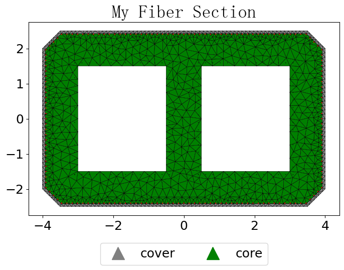
✨ RC section mesh#
Here we regard the RC section as a single-material section, ignoring the different material properties of steel bars and concrete.
[11]:
import numpy as np
import openseespy.opensees as ops
import opstool as opst
Generate geometric objects#
Functions: offset() and add_polygon() are used.
[12]:
# the points of the outer contour line, only the turning point of the line is needed, counterclockwise or clockwise.
outlines = [[0.5, 0], [7.5, 0], [8, 0.5], [8, 4.5],
            [7.5, 5], [0.5, 5], [0, 4.5], [0, 0.5]]
# cover thick
cover_d = 0.08
# Offset to get the inner boundary of the cover layer
coverlines = opst.offset(outlines, d=cover_d)

# Generate polygonal geometry object for cover layer
cover = opst.add_polygon(outlines, holes=[coverlines])

# Creating core with voids
holelines1 = [[1, 1], [3.5, 1], [3.5, 4], [1, 4]]
holelines2 = [[4.5, 1], [7, 1], [7, 4], [4.5, 4]]
core = opst.add_polygon(coverlines, holes=[holelines1, holelines2])
Generate mesh#
by class SecMesh.
[13]:
sec = opst.SecMesh(sec_name="My Fiber Section")
# Grouping, the dict key is the group name, which can be arbitrary.
sec.assign_group(dict(cover=cover, core=core))
# Specify the grid size
sec.assign_mesh_size(dict(cover=0.2, core=0.4))
sec.assign_group_color(dict(cover="gray", core="green"))
# Specify the material tag in the opensees, the material needs to be defined by you beforehand.
ops.uniaxialMaterial('Concrete01', 1, -30, -0.002, -15, -0.005)
ops.uniaxialMaterial('Concrete01', 2, -40, -0.006, -30, -0.015)
sec.assign_ops_matTag(dict(cover=1, core=2))
# mesh!
sec.mesh()
add rebars#
by class Rebars.
[29]:
ops.uniaxialMaterial('Steel01', 3, 200, 2.E5, 0.02)
# Instantiating the rebar class
rebars = opst.Rebars()

rebar_d_outer = 0.032   # dia of rebar
rebar_d_inner = 0.02
# Offset to obtain the rebars arranged along the contour line, Inward offset is positive
rebar_lines1 = opst.offset(outlines, d=cover_d + rebar_d_outer / 2)
# add the rebar line, gap is the spacing of the rebars, matTag is the opensees material tag predefined.
rebars.add_rebar_line(
    points=rebar_lines1, dia=rebar_d_outer, gap=0.15, color="red", matTag=3
)
# Offset to obtain the rebars arranged along the holes
rebar_lines2 = opst.offset(holelines1, d=-(cover_d + rebar_d_inner / 2))
rebars.add_rebar_line(
    points=rebar_lines2, dia=rebar_d_inner, gap=0.2, color="black", matTag=3
)
rebar_lines3 = opst.offset(holelines2, d=-(cover_d + rebar_d_inner / 2))
rebars.add_rebar_line(
    points=rebar_lines3, dia=rebar_d_inner, gap=0.2, color="black", matTag=3
)
[15]:
# add to the sec
sec.add_rebars(rebars)
Get the section properties#
section props dict, including:
Cross-sectional area (A)
Shear area (Asy, Asz)
Elastic centroid (centroid)
Second moments of area about the centroidal axis (Iy, Iz, Iyz)
Torsion constant (J)
Principal axis angle (phi)
ratio of reinforcement (rho_rebar)
Effective Material Properties (Effective elastic modulus: E_eff; Effective shear modulus: G_eff; Effective Poisson’s ratio: Nu_eff)
Tip
Since the finite element method is used to calculate the section properties by sectionproperties pacakge, the calculation may be a bit slow, which can be ignored if there is no need to calculate the section properties.
[16]:
sec_props = sec.get_sec_props(display_results=True, plot_centroids=False)
# for key, value in sec_props.items():
#     print(f"{key}: {value}")
                    Section Properties
┏━━━━━━━━━━━┳━━━━━━━━━━━━━━━━┳━━━━━━━━━━━━━━━━━━━━━━━━━━━┓
┃ Symbol    ┃ Value          ┃ Definition                ┃
┡━━━━━━━━━━━╇━━━━━━━━━━━━━━━━╇━━━━━━━━━━━━━━━━━━━━━━━━━━━┩
│ A         │ 24.500         │ Cross-sectional area      │
│ Asy       │ 13.963         │ Shear area y-axis         │
│ Asz       │ 12.119         │ Shear area z-axis         │
│ centroid  │ (4.000, 2.500) │ Elastic centroid          │
│ Iy        │ 69.354         │ Moment of inertia y-axis  │
│ Iz        │ 152.229        │ Moment of inertia z-axis  │
│ Iyz       │ 0.000          │ Product of inertia        │
│ J         │ 158.253        │ Torsion constant          │
│ phi       │ -90.000        │ Principal axis angle      │
│ rho_rebar │ 0.007          │ Ratio of reinforcement    │
│ E_eff     │ 1.000          │ Effective elastic modulus │
│ G_eff     │ 0.500          │ Effective shear modulus   │
│ Nu_eff    │ 0.000          │ Effective Poisson’s ratio │
└───────────┴────────────────┴───────────────────────────┘
centering or rotate the section#
[17]:
sec.centring()
#sec.rotate(90)
View the section mesh#
engine=’plotly’
[18]:
sec.view(fill=True, engine='plotly', save_html=None, on_notebook=True)
and engine=‘matplotlib’
[19]:
sec.view(fill=True, engine='matplotlib')
Generate py or tcl file#
[20]:
G = 10000   # Shear modulus
sec.to_file("mysec.py", secTag=1, GJ=G * sec_props['J'])
# sec.to_file("mysec.tcl", secTag=1, GJ=G * sec_props['J'])
Generate openseespy cmds implicitly#
This command can be used after defining the OpenSees material.
G = 10000   # Shear modulus
sec.opspy_cmds(secTag=1, GJ=G * sec_props['J'])
It’s done, you don’t need to do anything more.
✨ Composite Section Mesh#
Of course, we can also build composite material fiber sections, we need to use function add_material().
[1]:
import numpy as np
import opstool as opst
Specify the characteristics of each material
[3]:
Ec = 3.45E7
Es = 2.0E8
Nus = 0.3
Nuc = 0.2
steel_mat = opst.add_material(name='steel', elastic_modulus=Es, poissons_ratio=Nus)
conc_mat = opst.add_material(name='conc', elastic_modulus=Ec, poissons_ratio=Nuc)
Use predefined materials when generating geometric objects
[4]:
outlines = [[0, 0], [2, 0], [2, 2], [0, 2]]
coverlines = opst.offset(outlines, d=0.05)
cover = opst.add_polygon(outlines, holes=[coverlines], material=conc_mat)
bonelines = [[0.5, 0.5], [1.5, 0.5], [1.5, 0.7], [1.1, 0.7], [1.1, 1.3], [1.5, 1.3], [1.5, 1.5],
             [0.5, 1.5], [0.5, 1.3], [0.9, 1.3], [0.9, 0.7], [0.5, 0.7], [0.5, 0.5]]
core = opst.add_polygon(coverlines, holes=[bonelines], material=conc_mat)
bone = opst.add_polygon(bonelines, material=steel_mat)
mesh
[8]:
sec = opst.SecMesh()
sec.assign_group(dict(cover=cover, core=core, bone=bone))
sec.assign_mesh_size(dict(cover=0.02, core=0.05, bone=0.02))
sec.assign_group_color(dict(cover="gray", core="#b84592", bone='#ffc168'))
sec.assign_ops_matTag(dict(cover=1, core=2, bone=4))
sec.mesh()
add rebars
[9]:
# add rebars
rebars = opst.Rebars()
rebar_lines1 = opst.offset(outlines, d=0.05 + 0.032 / 2)
rebars.add_rebar_line(
    points=rebar_lines1, dia=0.032, gap=0.1, color="red", matTag=3
)
# add to the sec
sec.add_rebars(rebars)
Important
Use the modulus of elasticity to convert the geometric properties of the composite section into the equivalent properties of the reference material. Here, steel bar.
[7]:
sec_props = sec.get_sec_props(Eref=Es, display_results=True)
                    Section Properties
┏━━━━━━━━━━━┳━━━━━━━━━━━━━━━━┳━━━━━━━━━━━━━━━━━━━━━━━━━━━┓
┃ Symbol    ┃ Value          ┃ Definition                ┃
┡━━━━━━━━━━━╇━━━━━━━━━━━━━━━━╇━━━━━━━━━━━━━━━━━━━━━━━━━━━┩
│ A         │ 1.120          │ Cross-sectional area      │
│ Asy       │ 0.923          │ Shear area y-axis         │
│ Asz       │ 0.786          │ Shear area z-axis         │
│ centroid  │ (1.000, 1.000) │ Elastic centroid          │
│ Iy        │ 0.287          │ Moment of inertia y-axis  │
│ Iz        │ 0.258          │ Moment of inertia z-axis  │
│ Iyz       │ -0.000         │ Product of inertia        │
│ J         │ 0.428          │ Torsion constant          │
│ phi       │ 0.000          │ Principal axis angle      │
│ rho_rebar │ 0.052          │ Ratio of reinforcement    │
│ E_eff     │ 56015000.000   │ Effective elastic modulus │
│ G_eff     │ 22506250.000   │ Effective shear modulus   │
│ Nu_eff    │ 0.244          │ Effective Poisson’s ratio │
└───────────┴────────────────┴───────────────────────────┘
[10]:
sec.centring()
sec.view(fill=True, engine='plotly', save_html=None, on_notebook=True)
output the file
[28]:
Gs = Es / 2 / (1 + Nus)
sec.to_file("mysec.py", secTag=1, GJ=Gs * sec_props['J'])
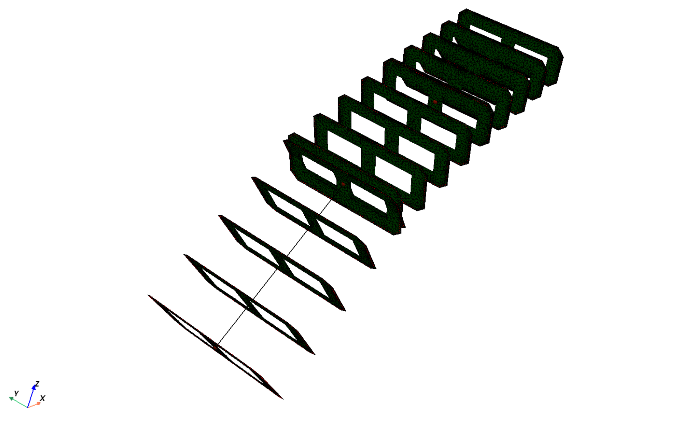
✨ Variable section mesh#
[5]:
import numpy as np
import opstool as opst
Function: var_line_string() is used to generate geometric line points that vary linearly or parabolicly, and then generate a cross-sectional mesh.
First determine the geometric data at both ends.
[10]:
# I end
outlines1 = [[0.5, 0], [7.5, 0], [8, 0.5], [8, 4.5],
            [7.5, 5], [0.5, 5], [0, 4.5], [0, 0.5]]
cover_d = 0.08
coverlines1 = opst.offset(outlines1, d=cover_d)
holelines1i = [[1, 1], [3.5, 1], [3.5, 4], [1, 4]]
holelines2i = [[4.5, 1], [7, 1], [7, 4], [4.5, 4]]
# J end
outlines2 = [[0.5, 0], [7.5, 0], [8, 0.5], [8, 2.5],
             [7.5, 3], [0.5, 3], [0, 2.5], [0, 0.5]]
cover_d = 0.05
coverlines2 = opst.offset(outlines2, d=cover_d)
holelines1j = [[1, 1], [3.5, 1], [3.5, 2], [1, 2]]
holelines2j = [[4.5, 1], [7, 1], [7, 2], [4.5, 2]]
To define a path of a section normal, it is recommended to determine a beam element every two coordinate points, where n_sec can be the number of fiber section integration points for each beam element.
[11]:
path = [(0, 0, 0), (8, 0, 8), (16, 0, 12), (24, 0, 15)] # 3 beam elements
Get geometric data at each integration point.
[12]:
outlines = opst.var_line_string(pointsi=outlines1, pointsj=outlines2,
                                path=path, n_sec=5, closure=True,
                                y_degree=1, y_sym_plane="j-0",
                                z_degree=2, z_sym_plane="j-0")
coverlines = opst.var_line_string(pointsi=coverlines1, pointsj=coverlines2,
                                  path=path, n_sec=5, closure=True,
                                  y_degree=1, y_sym_plane="j-0",
                                  z_degree=2, z_sym_plane="j-0")
holelines1 = opst.var_line_string(pointsi=holelines1i, pointsj=holelines1j,
                                  path=path, n_sec=5, closure=True,
                                  y_degree=1, y_sym_plane="j-0",
                                  z_degree=2, z_sym_plane="j-0")
holelines2 = opst.var_line_string(pointsi=holelines2i, pointsj=holelines2j,
                                  path=path, n_sec=5, closure=True,
                                  y_degree=1, y_sym_plane="j-0",
                                  z_degree=2, z_sym_plane="j-0")
Generate the section mesh at each integration point.
[15]:
sec_meshes = []
for i in range(len(outlines)):
    cover = opst.add_polygon(outlines[i], holes=[coverlines[i]])
    core = opst.add_polygon(coverlines[i], holes=[holelines1[i], holelines2[i]])
    sec = opst.SecMesh(sec_name=f"Section{i+1}")
    sec.assign_group(dict(cover=cover, core=core))
    sec.assign_mesh_size(dict(cover=0.2, core=0.4))
    sec.assign_group_color(dict(cover="gray", core="green"))
    sec.assign_ops_matTag(dict(cover=1, core=2))
    # mesh!
    sec.mesh()
    rebars = opst.Rebars()
    rebar_d_outer = 0.06   # dia of rebar
    rebar_d_inner = 0.06
    rebar_lines1 = opst.offset(coverlines[i], d=rebar_d_outer / 2)
    rebars.add_rebar_line(points=rebar_lines1, dia=rebar_d_outer,
                          gap=0.15, color="red", matTag=3)
    rebar_lines2 = opst.offset(holelines1[i], d=-(cover_d + rebar_d_inner / 2))
    rebars.add_rebar_line(
        points=rebar_lines2, dia=rebar_d_inner, gap=0.2, color="black", matTag=3
    )
    rebar_lines3 = opst.offset(holelines2[i], d=-(cover_d + rebar_d_inner / 2))
    rebars.add_rebar_line(
        points=rebar_lines3, dia=rebar_d_inner, gap=0.2, color="black", matTag=3
    )
    sec.add_rebars(rebars)
    sec.centring()  # must here
    sec_meshes.append(sec)
Function: vis_var_sec() is used to visualize varied section meshes.
[9]:
opst.vis_var_sec(sec_meshes=sec_meshes, path=path,
                 n_sec=5, on_notebook=False)
You can also generate openseespy commands directly.
i = 0
for sec in sec_meshes:
    sec.opspy_cmds(secTag=i+1, GJ=1000000)
    i += 1