Eigenvalue Results
[25]:
import openseespy.opensees as ops
import opstool as opst
import matplotlib.pyplot as plt
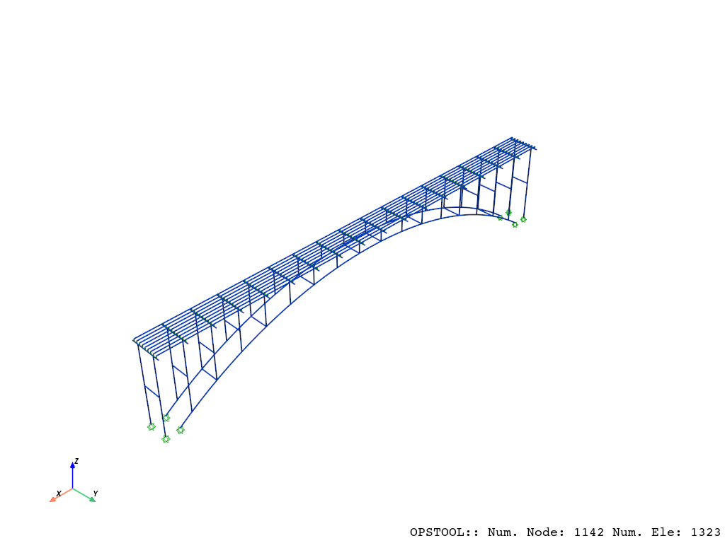
We use the built-in arch bridge example and visualize it:
[22]:
opst.load_ops_examples("ArchBridge")

# plot
opst.vis.pyvista.set_plot_props(notebook=True)
fig = opst.vis.pyvista.plot_model()
fig.show(jupyter_backend="static")
OPSTOOL :: Model data has been saved to _OPSTOOL_ODB/ModelData-None.nc!
Eigenvalue analysis data saving
API: opstool.post.save_eigen_data()
The following is our automatic analysis and saving of the data for the first 12 modes:
[3]:
opst.post.save_eigen_data(odb_tag=1, mode_tag=12)
Using DomainModalProperties - Developed by: Massimo Petracca, Guido Camata, ASDEA Software Technology
OPSTOOL :: Eigen data has been saved to _OPSTOOL_ODB/EigenData-1.nc!
Read the eigen data
API: opstool.post.get_eigen_data()
The following reads the saved data, noting that the odb_tag parameter is used to identify which result is being read
[4]:
model_props, eigen_vectors = opst.post.get_eigen_data(odb_tag=1)
OPSTOOL :: Loading eigen data from _OPSTOOL_ODB/EigenData-1.nc ...
Modal property data
Modal property data is saved as an xarray.DataArray structure, which facilitates more user-friendly data handling.
[5]:
model_props
[5]:
<xarray.DataArray 'ModalProps' (modeTags: 12, Properties: 34)> Size: 3kB
[408 values with dtype=float64]
Coordinates:
  * modeTags    (modeTags) int32 48B 1 2 3 4 5 6 7 8 9 10 11 12
  * Properties  (Properties) <U22 3kB 'eigenLambda' ... 'partiMassRatiosCumuRMY'
Attributes:
    domainSize:     3
    totalMass:      [4.36334920e+03 4.36334920e+03 4.36334920e+03 2.49393441e...
    totalFreeMass:  [4.23989360e+03 4.23989360e+03 4.23989360e+03 2.06174500e...
centerOfMass: [ 1.67585039e-17 2.55567185e-17 -1.69285810e+00]We can convert it into a pandas DataFrame for a more organized appearance:
[24]:
model_props_df = model_props.to_pandas()
model_props_df.head()
[24]:
| Properties | eigenLambda | eigenOmega | eigenFrequency | eigenPeriod | partiFactorMX | partiFactorMY | partiFactorRMZ | partiFactorMZ | partiFactorRMX | partiFactorRMY | ... | partiMassRatiosRMZ | partiMassRatiosMZ | partiMassRatiosRMX | partiMassRatiosRMY | partiMassRatiosCumuMX | partiMassRatiosCumuMY | partiMassRatiosCumuRMZ | partiMassRatiosCumuMZ | partiMassRatiosCumuRMX | partiMassRatiosCumuRMY |
|---|---|---|---|---|---|---|---|---|---|---|---|---|---|---|---|---|---|---|---|---|---|
| modeTags | |||||||||||||||||||||
| 1 | 21.816888 | 4.670855 | 0.743390 | 1.345189 | 1.305441e-10 | 5.787614e+01 | -1.697211e-08 | -3.794258e-11 | -1.503664e+02 | -4.976269e-09 | ... | 4.030547e-21 | 3.395462e-23 | 1.096647e+01 | 3.396501e-22 | 4.019382e-22 | 79.003097 | 4.030547e-21 | 3.395462e-23 | 10.966466 | 3.396501e-22 |
| 2 | 55.609654 | 7.457188 | 1.186848 | 0.842568 | 3.192704e+01 | -3.062447e-10 | -7.511326e-07 | 3.405789e-10 | 7.208872e-11 | -1.308159e+03 | ... | 7.894512e-18 | 2.735776e-21 | 2.520575e-24 | 2.347173e+01 | 2.404154e+01 | 79.003097 | 7.898543e-18 | 2.769730e-21 | 10.966466 | 2.347173e+01 |
| 3 | 56.147744 | 7.493180 | 1.192577 | 0.838521 | -1.036844e-08 | -3.770847e-10 | -2.329483e+03 | -2.446615e-11 | 1.420603e-09 | 4.228518e-07 | ... | 7.592960e+01 | 1.411810e-23 | 9.788370e-22 | 2.452452e-18 | 2.404154e+01 | 79.003097 | 7.592960e+01 | 2.783848e-21 | 10.966466 | 2.347173e+01 |
| 4 | 110.048060 | 10.490379 | 1.669596 | 0.598947 | -2.376746e-11 | -1.756824e+01 | -4.046576e-10 | 4.418021e-11 | 7.048508e+01 | 2.843537e-09 | ... | 2.291224e-24 | 4.603632e-23 | 2.409680e+00 | 1.109026e-22 | 2.404154e+01 | 86.282594 | 7.592960e+01 | 2.829885e-21 | 13.376147 | 2.347173e+01 |
| 5 | 167.129510 | 12.927858 | 2.057532 | 0.486019 | -4.080845e-10 | 1.466662e-10 | -4.120430e-09 | 1.323864e+01 | 1.085901e-09 | 1.374252e-08 | ... | 2.375621e-22 | 4.133632e+00 | 5.719338e-22 | 2.590340e-21 | 2.404154e+01 | 86.282594 | 7.592960e+01 | 4.133632e+00 | 13.376147 | 2.347173e+01 |
5 rows × 34 columns
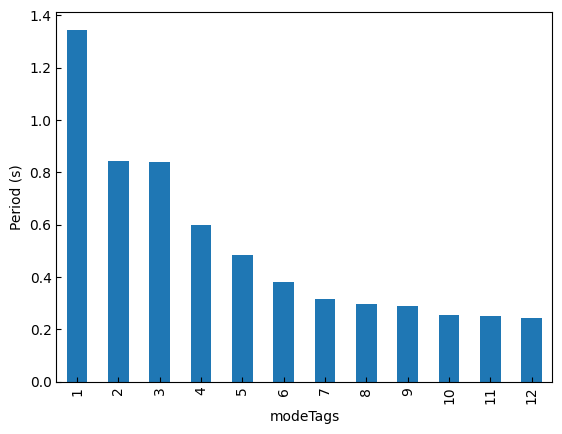
For example, we can index out the periods data:
[7]:
print(f"*** Eigen periods:\n {model_props_df["eigenPeriod"]}")
*** Eigen periods:
 modeTags
1     1.345189
2     0.842568
3     0.838521
4     0.598947
5     0.486019
6     0.382900
7     0.317327
8     0.296861
9     0.288235
10    0.253657
11    0.250341
12    0.244309
Name: eigenPeriod, dtype: float64
[28]:
periods = model_props_df["eigenPeriod"]
periods.plot.bar()
plt.ylabel("Period (s)")
plt.show()
For example, we can index out the cumulative mass participation ratio:
[8]:
keys = [
    "partiMassRatiosCumuMX",
    "partiMassRatiosCumuMY",
    "partiMassRatiosCumuMZ",
]
print(f"*** Cumulative participation mass ratio:\n {model_props_df[keys].head()}")
*** Cumulative participation mass ratio:
 Properties  partiMassRatiosCumuMX  partiMassRatiosCumuMY  \
modeTags
1                    4.019382e-22              79.003097
2                    2.404154e+01              79.003097
3                    2.404154e+01              79.003097
4                    2.404154e+01              86.282594
5                    2.404154e+01              86.282594

Properties  partiMassRatiosCumuMZ
modeTags
1                    3.395462e-23
2                    2.769730e-21
3                    2.783848e-21
4                    2.829885e-21
5                    4.133632e+00
Eigen vectors
In structural dynamics, eigenvectors play a crucial role in understanding the behavior of structures under dynamic loads. They provide insights into how a structure deforms or vibrates at specific natural frequencies (eigenvalues). These vectors, often referred to as mode shapes, are fundamental in modal analysis and dynamic response studies.
[9]:
eigen_vectors
[9]:
<xarray.DataArray 'EigenVectors' (modeTags: 12, nodeTags: 1142, DOFs: 6)> Size: 658kB
[82224 values with dtype=float64]
Coordinates:
  * modeTags  (modeTags) int32 48B 1 2 3 4 5 6 7 8 9 10 11 12
  * nodeTags  (nodeTags) int32 5kB 1 2 3 4 5 6 ... 1300 1301 1302 1303 1304 1305
  * DOFs      (DOFs) <U2 48B 'UX' 'UY' 'UZ' 'RX' 'RY' 'RZ'
You can retrieve dimension names in xarray.DataArray using the dims attribute:
[10]:
eigen_vectors.dims
[10]:
('modeTags', 'nodeTags', 'DOFs')
The .sel method can be used to retrieve specific elements corresponding to a particular dimension. For example, the following code helps us index the eigenvector at specific mode tags, node tags, and degrees of freedom.
[18]:
eigen_vectors_sub = eigen_vectors.sel(
    modeTags=[1, 2, 3, 4, 5], nodeTags=[100, 200, 300], DOFs=["UX", "UY", "UZ"]
)
eigen_vectors_sub
[18]:
<xarray.DataArray 'EigenVectors' (modeTags: 5, nodeTags: 3, DOFs: 3)> Size: 360B
[45 values with dtype=float64]
Coordinates:
  * modeTags  (modeTags) int32 20B 1 2 3 4 5
  * nodeTags  (nodeTags) int32 12B 100 200 300
  * DOFs      (DOFs) <U2 24B 'UX' 'UY' 'UZ'
Retrieve its data:
[19]:
eigen_vectors_sub.data
[19]:
array([[[ 2.63070107e-05,  1.86729203e-02, -1.52279473e-03],
        [-2.18801193e-04,  2.27953721e-02,  1.61430297e-03],
        [-7.49425264e-04,  1.24680018e-02, -6.84216416e-04]],

       [[ 1.07430986e-02, -1.06591436e-08,  1.86506167e-02],
        [ 7.95070024e-03, -2.17134681e-07,  1.26818563e-02],
        [ 7.36071603e-03,  1.19360223e-07, -7.40619716e-03]],

       [[ 1.20462762e-03, -7.55738596e-03,  1.80162219e-03],
        [-1.36398139e-03, -6.54061212e-03, -1.15008967e-03],
        [ 1.03647160e-03,  2.41749630e-02, -2.06422175e-03]],

       [[ 5.90844295e-04,  9.57100011e-03,  1.01994926e-03],
        [-7.27628557e-04,  1.14606700e-02, -4.73067678e-04],
        [-2.31617124e-03, -2.16609879e-02,  2.24017969e-03]],

       [[-1.99630301e-03, -9.49229075e-07,  1.41933100e-02],
        [ 2.35318153e-05, -6.52638665e-07,  2.62522766e-02],
        [-3.22705290e-04, -3.92921381e-08, -8.33629307e-03]]])