Shell element Response
[1]:
import numpy as np
import openseespy.opensees as ops
import opstool as opst
import matplotlib.pyplot as plt
[2]:
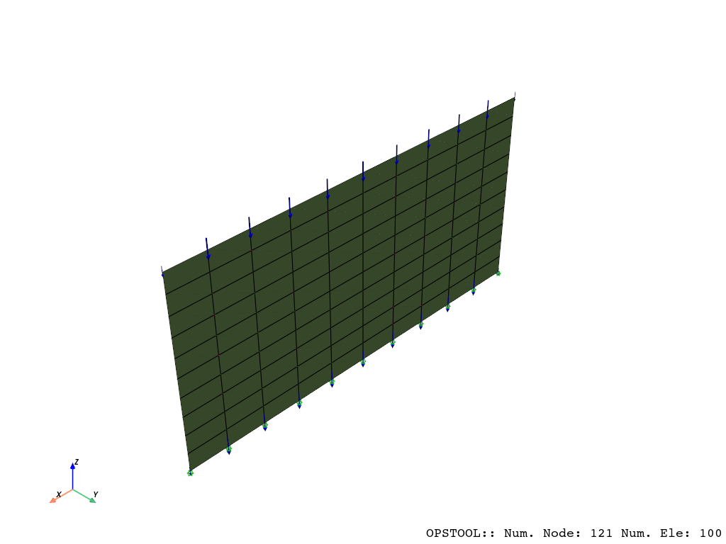
opst.load_ops_examples("Shell3D")  # or your model code here

# add beam loads
ops.timeSeries("Linear", 1)
ops.pattern("Plain", 1, 1)
opst.pre.gen_grav_load(direction="z", factor=-9810)


# plot
opst.vis.pyvista.set_plot_props(notebook=True)
fig = opst.vis.pyvista.plot_model(show_nodal_loads=True, show_ele_loads=True)
fig.show(jupyter_backend="static")
The original Tcl file comes from http://www.dinochen.com/, and the Python version is converted by opstool.tcl2py().
OPSTOOL :: Model data has been saved to _OPSTOOL_ODB/ModelData-None.nc!
Result Saving
[3]:
ops.system("BandGeneral")
# Create the constraint handler, the transformation method
ops.constraints("Transformation")
# Create the DOF numberer, the reverse Cuthill-McKee algorithm
ops.numberer("RCM")
# Create the convergence test, the norm of the residual with a tolerance of
# 1e-12 and a max number of iterations of 10
ops.test("NormDispIncr", 1.0e-12, 10, 3)
# Create the solution algorithm, a Newton-Raphson algorithm
ops.algorithm("Newton")
# Create the integration scheme, the LoadControl scheme using steps of 0.1
ops.integrator("LoadControl", 0.1)
# Create the analysis object
ops.analysis("Static")
opstool allows us to save the data at each step of the analysis!
First, we create a database class using opstool.post.CreateODB, and then, during each step of the analysis, we call its method .fetch_response_step to retrieve the data for the current step.
Once all the analysis steps are completed, we use the .save_response method to save the data in one go.
[4]:
ODB = opst.post.CreateODB(odb_tag=1)
for i in range(10):
    ops.analyze(1)
    ODB.fetch_response_step()
ODB.save_response()
OPSTOOL :: All responses data with odb_tag = 1 saved in _OPSTOOL_ODB/RespStepData-1.nc!
Result Reading
The provided function opstool.post.get_element_responses() make it easy to read element responses.
ele_type="Shell" is used to specify extracting the response of shell elements.
[5]:
all_resp = opst.post.get_element_responses(odb_tag=1, ele_type="Shell")
OPSTOOL :: Loading response data from _OPSTOOL_ODB/RespStepData-1.nc ...
The result is an xarray DataSet object, and we can access the associated DataArray objects through .data_vars.
[6]:
all_resp.data_vars
[6]:
Data variables:
    sectionForces        (time, eleTags, GaussPoints, secDOFs) float64 282kB ...
    sectionDeformations  (time, eleTags, GaussPoints, secDOFs) float64 282kB ...
    Stresses             (time, eleTags, GaussPoints, fiberPoints, stressDOFs) float64 880kB ...
    Strains              (time, eleTags, GaussPoints, fiberPoints, stressDOFs) float64 880kB ...
section forces and deformations at Gauss points are supported, representing the shell section response per unit length.
Stresses and Strains refer to the fiber stress and strain at the Gauss points. fiberPoints represents the fiber No. on each section at the Gauss point, typically counted from the bottom. Stress and strain have five components, because sigma33 (the normal stress along the local z-axis) is zero and omitted. The remaining components represent stresses along the local directions.
[7]:
all_resp.attrs # attributes
[7]:
{'FXX,FYY,FXY': 'Membrane (in-plane) forces or deformations.',
 'MXX,MYY,MXY': 'Bending moments or rotations (out-plane) of plate.',
 'VXZ,VYZ': 'Shear forces or deformations.',
 'sigma11, sigma22': 'Normal stress (strain) along local x, y',
 'sigma12, sigma23, sigma13': 'Shear stress (strain).'}
Section response
[8]:
sec_forces = all_resp["sectionForces"]
sec_forces
[8]:
<xarray.DataArray 'sectionForces' (time: 11, eleTags: 100, GaussPoints: 4,
                                   secDOFs: 8)> Size: 282kB
[35200 values with dtype=float64]
Coordinates:
  * eleTags      (eleTags) int32 400B 1 2 3 4 5 6 7 8 ... 94 95 96 97 98 99 100
  * GaussPoints  (GaussPoints) int32 16B 1 2 3 4
  * secDOFs      (secDOFs) <U3 96B 'FXX' 'FYY' 'FXY' 'MXX' ... 'MXY' 'VXZ' 'VYZ'
* time (time) float64 88B 0.0 0.1 0.2 0.3 0.4 0.5 0.6 0.7 0.8 0.9 1.0Let’s take a look at the various coordinates.
[9]:
sec_forces.coords
[9]:
Coordinates:
* eleTags (eleTags) int32 400B 1 2 3 4 5 6 7 8 ... 94 95 96 97 98 99 100
* GaussPoints (GaussPoints) int32 16B 1 2 3 4
* secDOFs (secDOFs) <U3 96B 'FXX' 'FYY' 'FXY' 'MXX' ... 'MXY' 'VXZ' 'VYZ'
* time (time) float64 88B 0.0 0.1 0.2 0.3 0.4 0.5 0.6 0.7 0.8 0.9 1.0
[10]:
sec_forces.coords["eleTags"].data # all element tags
[10]:
array([  1,   2,   3,   4,   5,   6,   7,   8,   9,  10,  11,  12,  13,  14,
        15,  16,  17,  18,  19,  20,  21,  22,  23,  24,  25,  26,  27,  28,
        29,  30,  31,  32,  33,  34,  35,  36,  37,  38,  39,  40,  41,  42,
        43,  44,  45,  46,  47,  48,  49,  50,  51,  52,  53,  54,  55,  56,
        57,  58,  59,  60,  61,  62,  63,  64,  65,  66,  67,  68,  69,  70,
        71,  72,  73,  74,  75,  76,  77,  78,  79,  80,  81,  82,  83,  84,
        85,  86,  87,  88,  89,  90,  91,  92,  93,  94,  95,  96,  97,  98,
        99, 100])
[11]:
sec_forces.coords["secDOFs"].data # all section DOFs
[11]:
array(['FXX', 'FYY', 'FXY', 'MXX', 'MYY', 'MXY', 'VXZ', 'VYZ'],
      dtype='<U3')
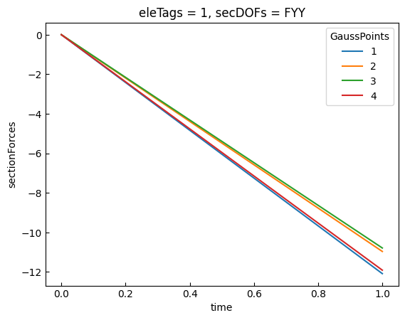
Below, we select the membrane force \(F_{YY}\) of element 1.
[12]:
sec_forces_fxx = sec_forces.sel(
    eleTags=1,
    secDOFs="FYY",
)
# plot
sec_forces_fxx.plot.line(
    x="time",
)
plt.show()
Stresses and Strains
Below, we retrieve the stress and strain data, which is a five-dimensional array. The dimensions are, in order, (‘time’, ‘eleTags’, ‘GaussPoints’, ‘fiberPoints’, ‘stressDOFs’), and we can conveniently retrieve data based on these dimensions and their coordinates.
[13]:
stresses = all_resp["Stresses"]
strains = all_resp["Strains"]
print(stresses)
print("=" * 100)
print(strains)
print("=" * 100)
print(stresses.dims)
<xarray.DataArray 'Stresses' (time: 11, eleTags: 100, GaussPoints: 4,
                              fiberPoints: 5, stressDOFs: 5)> Size: 880kB
[110000 values with dtype=float64]
Coordinates:
  * eleTags      (eleTags) int32 400B 1 2 3 4 5 6 7 8 ... 94 95 96 97 98 99 100
  * GaussPoints  (GaussPoints) int32 16B 1 2 3 4
  * fiberPoints  (fiberPoints) int32 20B 1 2 3 4 5
  * stressDOFs   (stressDOFs) <U7 140B 'sigma11' 'sigma22' ... 'sigma13'
  * time         (time) float64 88B 0.0 0.1 0.2 0.3 0.4 0.5 0.6 0.7 0.8 0.9 1.0
====================================================================================================
<xarray.DataArray 'Strains' (time: 11, eleTags: 100, GaussPoints: 4,
                             fiberPoints: 5, stressDOFs: 5)> Size: 880kB
[110000 values with dtype=float64]
Coordinates:
  * eleTags      (eleTags) int32 400B 1 2 3 4 5 6 7 8 ... 94 95 96 97 98 99 100
  * GaussPoints  (GaussPoints) int32 16B 1 2 3 4
  * fiberPoints  (fiberPoints) int32 20B 1 2 3 4 5
  * stressDOFs   (stressDOFs) <U7 140B 'sigma11' 'sigma22' ... 'sigma13'
  * time         (time) float64 88B 0.0 0.1 0.2 0.3 0.4 0.5 0.6 0.7 0.8 0.9 1.0
====================================================================================================
('time', 'eleTags', 'GaussPoints', 'fiberPoints', 'stressDOFs')
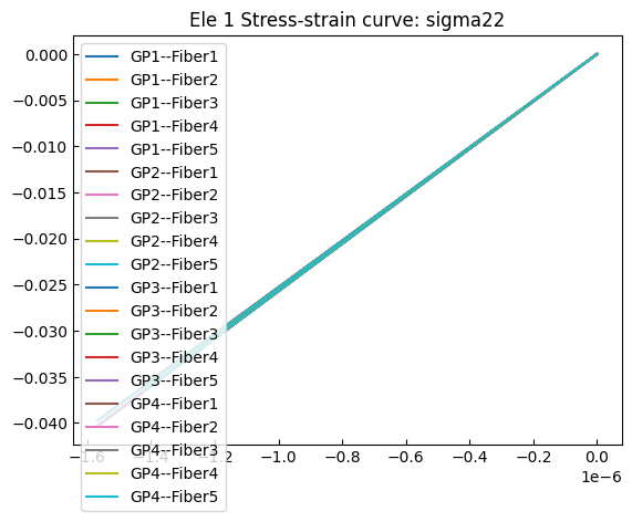
[14]:
stresses2 = stresses.sel(eleTags=1, stressDOFs="sigma22")
strains2 = strains.sel(eleTags=1, stressDOFs="sigma22")
gauss_points = stresses2.coords["GaussPoints"].data
fiber_points = stresses2.coords["fiberPoints"].data
[15]:
for gp_no in gauss_points:
    for fiber_no in fiber_points:
        s = stresses2.sel(GaussPoints=gp_no, fiberPoints=fiber_no)
        d = strains2.sel(GaussPoints=gp_no, fiberPoints=fiber_no)
        plt.plot(d, s, label=f"GP{gp_no}--Fiber{fiber_no}")
plt.title("Ele 1 Stress-strain curve: sigma22")
plt.legend()
plt.show()
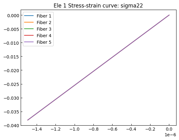
We can also compute averages along a specific dimension. For example, below, we calculate the average stress at the Gauss points:
[16]:
stresses3 = stresses2.mean(dim="GaussPoints")
strains3 = strains2.mean(dim="GaussPoints")

for fiber_no in fiber_points:
    s = stresses3.sel(fiberPoints=fiber_no)
    d = strains3.sel(fiberPoints=fiber_no)
    plt.plot(d, s, label=f"Fiber {fiber_no}")
plt.title("Ele 1 Stress-strain curve: sigma22")
plt.legend()
plt.show()