Planar element response¶

Original code see: Solid-fluid fully coupled (u-p) plane-strain 9-4 noded element: saturated soil element with pressure dependent material, subjected to 1D sinusoidal base shaking

[1]:

import numpy as np
import matplotlib.pyplot as plt
import openseespy.opensees as ops
import opstool as opst

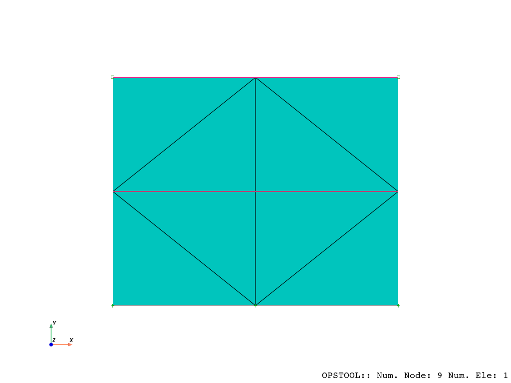
Model¶

[2]:

ops.wipe()
ops.model("basic", "-ndm", 2, "-ndf", 3)
ops.node(1, 0, 0)
ops.node(2, 2.5, 0)
ops.node(3, 2.5, 2)
ops.node(4, 0, 2)
ops.fix(1, 1, 1, 0)
ops.fix(2, 1, 1, 0)
ops.fix(3, 0, 0, 1)
ops.fix(4, 0, 0, 1)
ops.equalDOF(3, 4, 1, 2)
ops.model("basic", "-ndm", 2, "-ndf", 2)
ops.node(5, 1.25, 0.0)
ops.node(6, 2.5, 1)
ops.node(7, 1.25, 2)
ops.node(8, 0, 1)
ops.node(9, 1.25, 1)
ops.fix(5, 1, 1)
ops.equalDOF(3, 7, 1, 2)
ops.equalDOF(6, 8, 1, 2)
ops.equalDOF(6, 9, 1, 2)
ops.nDMaterial(
    "PressureDependMultiYield02", 1, 2, 1.8, 90000.0, 220000.0, 32, 0.1, 80, 0.5, 26.0, 0.067, 0.23, 0.06, 0.27
)
ops.element(
    "9_4_QuadUP",
    1,
    1,
    2,
    3,
    4,
    5,
    6,
    7,
    8,
    9,
    1.0,
    1,
    2200000.0,
    1,
    5.096839959225281e-07,
    5.096839959225281e-07,
    0.0,
    -9.81,
)

[3]:

opsvis = opst.vis.pyvista

opsvis.set_plot_props(notebook=True)
fig = opsvis.plot_model()
fig.show(jupyter_backend="jupyterlab")

OPSTOOL ::  Model data has been saved to _OPSTOOL_ODB/ModelData-None.nc!

../../_images/src_post_plane_up_resp_5_1.png

GRAVITY APPLICATION (elastic behavior)¶

[4]:

# create the SOE, ConstraintHandler, Integrator, Algorithm and Numberer
ops.updateMaterialStage("-material", 1, "-stage", 0)
ops.numberer("RCM")
ops.system("ProfileSPD")
ops.test("NormDispIncr", 1e-08, 30, 0)
ops.algorithm("KrylovNewton")
ops.constraints("Penalty", 1e18, 1e18)
ops.integrator("Newmark", 1.5, 1.0)
ops.analysis("Transient")
ops.analyze(10, 5000.0)
ops.updateMaterialStage("-material", 1, "-stage", 1)
ops.analyze(100, 1.0)

[4]:

APPLY LOADING SEQUENCE AND ANALYZE (plastic)¶

[5]:

ops.wipeAnalysis()
ops.setTime(0.0)
ops.timeSeries("Trig", 1, 0.0, 10.0, 1.0, "-factor", 2)
ops.pattern("UniformExcitation", 1, 1, "-accel", 1)

[6]:

ops.constraints("Penalty", 1e18, 1e18)
ops.test("NormDispIncr", 0.0001, 25, 0)
ops.numberer("RCM")
ops.algorithm("KrylovNewton")
ops.system("ProfileSPD")
ops.integrator("Newmark", 0.6, 0.30250000000000005)
ops.rayleigh(0.0, 0.0, 0.002, 0.0)
ops.analysis("Transient")

Save the results¶

[7]:

ODB = opst.post.CreateODB(odb_tag=1)
for _ in range(2500):
    ops.analyze(1, 0.01)
    ODB.fetch_response_step()
ODB.save_response(zlib=True)

OPSTOOL ::  All responses data with _odb_tag = 1 saved in _OPSTOOL_ODB/RespStepData-1.nc!

Post-processing¶

Nodal responses¶

[8]:

node_resp = opst.post.get_nodal_responses(odb_tag=1)
print(node_resp)

OPSTOOL ::  Loading all response data from _OPSTOOL_ODB/RespStepData-1.nc ...

<xarray.Dataset> Size: 7MB
Dimensions:             (time: 2501, nodeTags: 9, DOFs: 6)
Coordinates:
  * nodeTags            (nodeTags) int32 36B 1 2 3 4 5 6 7 8 9
  * DOFs                (DOFs) <U2 48B 'UX' 'UY' 'UZ' 'RX' 'RY' 'RZ'
  * time                (time) float64 20kB 0.0 0.01 0.02 ... 24.98 24.99 25.0
Data variables:
    disp                (time, nodeTags, DOFs) float64 1MB -9.002e-18 ... 0.0
    vel                 (time, nodeTags, DOFs) float64 1MB -2.549e-29 ... 0.0
    accel               (time, nodeTags, DOFs) float64 1MB 9.82e-31 ... 0.0
    reaction            (time, nodeTags, DOFs) float64 1MB 2.462 7.903 ... 0.0
    reactionIncInertia  (time, nodeTags, DOFs) float64 1MB 9.002 14.72 ... 0.0
    rayleighForces      (time, nodeTags, DOFs) float64 1MB -4.713e-14 ... 0.0
    pressure            (time, nodeTags) float32 90kB 0.0 0.0 0.0 ... 0.0 0.0
Attributes:
    UX:       Displacement in X direction
    UY:       Displacement in Y direction
    UZ:       Displacement in Z direction
    RX:       Rotation about X axis
    RY:       Rotation about Y axis
    RZ:       Rotation about Z axis

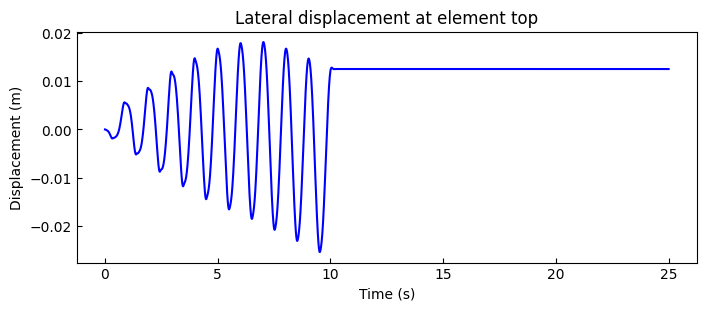
node 3 displacement relative to node 1¶

[9]:

disp1 = node_resp["disp"].sel(nodeTags=1, DOFs="UX")
disp3 = node_resp["disp"].sel(nodeTags=3, DOFs="UX")
times = node_resp["time"].data

fig, ax = plt.subplots(1, 1, figsize=(8, 3))
ax.plot(times, disp3 - disp1, "b")
ax.set_title("Lateral displacement at element top")
ax.set_xlabel("Time (s)")
ax.set_ylabel("Displacement (m)")
plt.show()

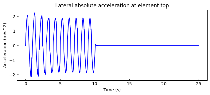
../../_images/src_post_plane_up_resp_17_0.png

node 3 acceleration¶

[10]:

from scipy.interpolate import interp1d


t = np.linspace(0, 20 * np.pi, int(20 * np.pi / (np.pi / 50)) + 1)
s = 2 * np.sin(t)
s = np.concatenate((s, np.zeros(3000)))
x_original = np.linspace(0, 40, len(s))
interp_func = interp1d(x_original, s, kind="linear", fill_value="extrapolate")
s1 = interp_func(times)

[11]:

acc3 = node_resp["accel"].sel(nodeTags=3, DOFs="UX")
times = node_resp["time"].data

fig, ax = plt.subplots(1, 1, figsize=(8, 3))
ax.plot(times, s1 + acc3, "b")
ax.set_title("Lateral absolute acceleration at element top")
ax.set_xlabel("Time (s)")
ax.set_ylabel("Acceleration (m/s^2)")
plt.show()

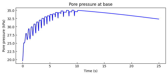
../../_images/src_post_plane_up_resp_20_0.png

Pore pressure at base¶

[12]:

p1 = node_resp["vel"].sel(nodeTags=1, DOFs="RZ")

fig, ax = plt.subplots(1, 1, figsize=(8, 3))

ax.plot(times, p1, "b")
ax.set_title("Pore pressure at base")
ax.set_xlabel("Time (s)")
ax.set_ylabel("Pore pressure (kPa)")
plt.show()

../../_images/src_post_plane_up_resp_22_0.png

Elemental response¶

[13]:

ele_resp = opst.post.get_element_responses(odb_tag=1, ele_type="Plane")
print(ele_resp)

OPSTOOL ::  Loading Plane response data from _OPSTOOL_ODB/RespStepData-1.nc ...

<xarray.Dataset> Size: 3MB
Dimensions:         (time: 2501, eleTags: 1, GaussPoints: 9, stressDOFs: 5,
                     strainDOFs: 3, measures: 4)
Coordinates:
  * eleTags         (eleTags) int32 4B 1
  * GaussPoints     (GaussPoints) int32 36B 1 2 3 4 5 6 7 8 9
  * stressDOFs      (stressDOFs) <U7 140B 'sigma11' 'sigma22' ... 'eta_r'
  * strainDOFs      (strainDOFs) <U5 60B 'eps11' 'eps22' 'eps12'
  * time            (time) float64 20kB 0.0 0.01 0.02 0.03 ... 24.98 24.99 25.0
  * measures        (measures) <U8 128B 'p1' 'p2' 'sigma_vm' 'tau_max'
Data variables:
    Stresses        (time, eleTags, GaussPoints, stressDOFs) float64 900kB -6...
    Strains         (time, eleTags, GaussPoints, strainDOFs) float64 540kB 1....
    stressMeasures  (time, eleTags, GaussPoints, measures) float64 720kB -6.5...
    strainMeasures  (time, eleTags, GaussPoints, measures) float32 360kB 1.22...
Attributes:
    p1, p2:                     Principal stresses (strains).
    sigma11, sigma22, sigma12:  Normal stress and shear stress (strain) in th...
    eta_r:                      Ratio between the shear (deviatoric) stress a...
    sigma_vm:                   Von Mises stress.
    tau_max:                    Maximum shear stress (strains).

Extract the stresses of element 1

[14]:

sigma11 = ele_resp["Stresses"].sel(stressDOFs="sigma11", eleTags=1)
sigma22 = ele_resp["Stresses"].sel(stressDOFs="sigma22", eleTags=1)
sigma33 = ele_resp["Stresses"].sel(stressDOFs="sigma33", eleTags=1)
sigma12 = ele_resp["Stresses"].sel(stressDOFs="sigma12", eleTags=1)
eta_r = ele_resp["Stresses"].sel(stressDOFs="eta_r", eleTags=1)

Calculate confinement p and deviatoric stress q

[15]:

po = (sigma11 + sigma22 + sigma33) / 3.0
qo = (sigma11 - sigma22) ** 2 + (sigma22 - sigma33) ** 2 + (sigma33 - sigma11) ** 2 + 6 * (sigma12**2)
qo = np.sign(sigma12) * 1 / 3 * np.sqrt(qo)
print(qo)

<xarray.DataArray 'Stresses' (time: 2501, GaussPoints: 9)> Size: 180kB
array([[-3.47572964,  3.47572964, -0.44147555, ..., -0.44147555,
         1.9586026 ,  1.9586026 ],
       [-3.47460759, -3.47460759, -0.44140656, ..., -0.44140656,
        -1.95825618, -1.95825618],
       [-3.46950994, -3.46950994, -0.44015566, ..., -0.44015566,
        -1.95585671, -1.95585671],
       ...,
       [-0.50187619, -0.50187619, -0.07121333, ..., -0.07121333,
         0.26772495,  0.26772495],
       [-0.50228011, -0.50228011, -0.07127072, ..., -0.07127072,
         0.26793408,  0.26793408],
       [-0.50268413, -0.50268413, -0.07132813, ..., -0.07132813,
         0.26814326,  0.26814326]])
Coordinates:
    eleTags      int32 4B 1
  * GaussPoints  (GaussPoints) int32 36B 1 2 3 4 5 6 7 8 9
    stressDOFs   <U7 28B 'sigma12'
  * time         (time) float64 20kB 0.0 0.01 0.02 0.03 ... 24.98 24.99 25.0

Extract the strains of element 1

[16]:

eps11 = ele_resp["Strains"].sel(strainDOFs="eps11", eleTags=1)
eps22 = ele_resp["Strains"].sel(strainDOFs="eps22", eleTags=1)
eps12 = ele_resp["Strains"].sel(strainDOFs="eps12", eleTags=1)

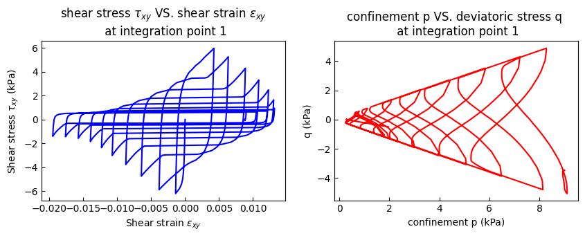
integration point 1 p-q¶

[17]:

eps12_ele1_1 = eps12.sel(GaussPoints=1)
sigma12_ele1_1 = sigma12.sel(GaussPoints=1)
po_ele1_1 = po.sel(GaussPoints=1)
qo_ele1_1 = qo.sel(GaussPoints=1)

fig, axs = plt.subplots(1, 2, figsize=(10, 3))
axs[0].plot(eps12_ele1_1, sigma12_ele1_1, "b")
axs[0].set_title("shear stress $\\tau_{xy}$ VS. shear strain $\\epsilon_{xy}$ \n at integration point 1")
axs[0].set_xlabel(r"Shear strain $\epsilon_{xy}$")
axs[0].set_ylabel(r"Shear stress $\tau_{xy}$ (kPa)")
axs[1].plot(-po_ele1_1, qo_ele1_1, "r")
axs[1].set_title("confinement p VS. deviatoric stress q \n at integration point 1")
axs[1].set_xlabel("confinement p (kPa)")
axs[1].set_ylabel("q (kPa)")
plt.show()

../../_images/src_post_plane_up_resp_32_0.png

integration point 5 p-q¶

[18]:

eps12_ele1_5 = eps12.sel(GaussPoints=5)
sigma12_ele1_5 = sigma12.sel(GaussPoints=5)
po_ele1_5 = po.sel(GaussPoints=5)
qo_ele1_5 = qo.sel(GaussPoints=5)

fig, axs = plt.subplots(1, 2, figsize=(10, 3))
axs[0].plot(eps12_ele1_5, sigma12_ele1_5, "b")
axs[0].set_title("shear stress $\\tau_{xy}$ VS. shear strain $\\epsilon_{xy}$ \n at integration point 5")
axs[0].set_xlabel(r"Shear strain $\epsilon_{xy}$")
axs[0].set_ylabel(r"Shear stress $\tau_{xy}$ (kPa)")
axs[1].plot(-po_ele1_5, qo_ele1_5, "r")
axs[1].set_title("confinement p VS. deviatoric stress q \n at integration point 5")
axs[1].set_xlabel("confinement p (kPa)")
axs[1].set_ylabel("q (kPa)")
plt.show()

../../_images/src_post_plane_up_resp_34_0.png

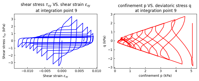
integration point 9 p-q¶

[19]:

eps12_ele1_9 = eps12.sel(GaussPoints=9)
sigma12_ele1_9 = sigma12.sel(GaussPoints=9)
po_ele1_9 = po.sel(GaussPoints=9)
qo_ele1_9 = qo.sel(GaussPoints=9)

fig, axs = plt.subplots(1, 2, figsize=(10, 3))
axs[0].plot(eps12_ele1_9, sigma12_ele1_9, "b")
axs[0].set_title("shear stress $\\tau_{xy}$ VS. shear strain $\\epsilon_{xy}$ \n at integration point 9")
axs[0].set_xlabel(r"Shear strain $\epsilon_{xy}$")
axs[0].set_ylabel(r"Shear stress $\tau_{xy}$ (kPa)")
axs[1].plot(-po_ele1_9, qo_ele1_9, "r")
axs[1].set_title("confinement p VS. deviatoric stress q \n at integration point 9")
axs[1].set_xlabel("confinement p (kPa)")
axs[1].set_ylabel("q (kPa)")
plt.show()

../../_images/src_post_plane_up_resp_36_0.png