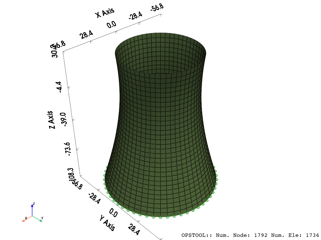
Modal analysis of a cooling tower
Gmsh model
You can find modeling instructions at: Creating quadrilateral surface meshes with gmsh

[47]:
import gmsh
import sys
import math
import json
[48]:
# Initialize gmsh
gmsh.initialize()

gmsh.model.add("forma11c_gmsh")
forma11c_profile.json can be downloaded from here
[49]:
# Read the profile coordinates
file_id = open("forma11c_profile.json", "r")
coords = json.load(file_id)
file_id.close()
[50]:
# Set a default element size
el_size = 1.0

# Add profile points
v_profile = []
for coord in coords:
    v = gmsh.model.occ.addPoint(coord[0], coord[1], coord[2], el_size)
    v_profile.append(v)
[51]:
# Add spline going through profile points
l1 = gmsh.model.occ.addBSpline(v_profile)
# Create copies and rotate
l2 = gmsh.model.occ.copy([(1, l1)])
l3 = gmsh.model.occ.copy([(1, l1)])
l4 = gmsh.model.occ.copy([(1, l1)])

# Rotate the copy
gmsh.model.occ.rotate(l2, 0, 0, 0, 0, 0, 1, math.pi / 2)
gmsh.model.occ.rotate(l3, 0, 0, 0, 0, 0, 1, math.pi)
gmsh.model.occ.rotate(l4, 0, 0, 0, 0, 0, 1, 3 * math.pi / 2)
[52]:
# Sweep the lines
surf1 = gmsh.model.occ.revolve([(1, l1)], 0, 0, 0, 0, 0, 1, math.pi / 2)
surf2 = gmsh.model.occ.revolve(l2, 0, 0, 0, 0, 0, 1, math.pi / 2)
surf3 = gmsh.model.occ.revolve(l3, 0, 0, 0, 0, 0, 1, math.pi / 2)
surf4 = gmsh.model.occ.revolve(l4, 0, 0, 0, 0, 0, 1, math.pi / 2)
[53]:
# Join the surfaces
surf5 = gmsh.model.occ.fragment(surf1, surf2)
surf6 = gmsh.model.occ.fragment(surf3, surf4)
surf7 = gmsh.model.occ.fragment(surf5[0], surf6[0])
[54]:
gmsh.model.occ.remove_all_duplicates()
gmsh.model.occ.synchronize()
[55]:
num_nodes_circ = 15
for curve in gmsh.model.occ.getEntities(1):
    gmsh.model.mesh.setTransfiniteCurve(curve[1], num_nodes_circ)
[56]:
num_nodes_vert = 32
vertical_curves = [7, 10, 13, 17]
for curve in vertical_curves:
    gmsh.model.mesh.setTransfiniteCurve(curve, num_nodes_vert)
[57]:
for surf in gmsh.model.occ.getEntities(2):
    gmsh.model.mesh.setTransfiniteSurface(surf[1])
[58]:
gmsh.option.setNumber("Mesh.RecombineAll", 1)
gmsh.option.setNumber("Mesh.RecombinationAlgorithm", 1)
gmsh.option.setNumber("Mesh.Recombine3DLevel", 2)
gmsh.option.setNumber("Mesh.ElementOrder", 1)
[59]:
# Important:
# Note that we use names to distinguish groups, so please do not overlook this!
# We use the "Boundary" group to include 4 lines
gmsh.model.addPhysicalGroup(dim=1, tags=[6, 9, 12, 15], tag=1, name="Boundary")
[59]:
1
[60]:
# Generate mesh
gmsh.model.mesh.generate(dim=2)
[61]:
gmsh.option.setNumber("Mesh.SaveAll", 1)
gmsh.write("forma11c.msh")
[62]:
gmsh.fltk.run()
To OpenSeesPy Model
[18]:
import openseespy.opensees as ops
import opstool as opst
[33]:
ops.wipe()
ops.model("basic", "-ndm", 3, "-ndf", 6)
E, nu, rho = 2.76e10, 0.166, 2244.0  # Pa, kg/m3
ops.nDMaterial("ElasticIsotropic", 1, E, nu, rho)
secTag = 11
ops.section("PlateFiber", secTag, 1, 0.305)
[34]:
GMSH2OPS = opst.pre.Gmsh2OPS(ndm=3, ndf=6)
[35]:
GMSH2OPS.read_gmsh_file("forma11c.msh")
Info:: 1 Physical Names.
Info:: 1821 Nodes; MaxNodeTag 1821; MinNodeTag 1.
Info:: 2009 Elements; MaxEleTag 2009; MinEleTag 1.
Info:: Geometry Information >>>
53 Entities: 37 Point; 12 Curves; 4 Surfaces; 0 Volumes.

Info:: Physical Groups Information >>>
1 Physical Groups.
Physical Group names: ['Boundary']

Info:: Mesh Information >>>
1821 Nodes; MaxNodeTag 1821; MinNodeTag 1.
1972 Elements; MaxEleTag 2009; MinEleTag 38.
[36]:
# Create OpenSeesPy node commands based on all nodes defined in the GMSH file
node_tags = GMSH2OPS.create_node_cmds()
[37]:
dim_entity_tags = GMSH2OPS.get_dim_entity_tags()
dim_entity_tags_2D = [item for item in dim_entity_tags if item[0] == 2]
[38]:
# Create OpenSeesPy element commands for specific entities
ele_tags_n4 = GMSH2OPS.create_element_cmds(
    ops_ele_type="ASDShellQ4",  # OpenSeesPy element type
    ops_ele_args=[
        secTag
    ],  # Additional arguments for the element (e.g., section tag)
    dim_entity_tags=dim_entity_tags_2D,
)
[39]:
boundary_dim_tags = GMSH2OPS.get_boundary_dim_tags(
    physical_group_names="Boundary", include_self=True)
boundary_dim_tags
[39]:
[(0, 55), (0, 59), (0, 61), (0, 63), (1, 6), (1, 9), (1, 12), (1, 15)]
[40]:
fix_ntags = GMSH2OPS.create_fix_cmds(dim_entity_tags=boundary_dim_tags,
                                     dofs=[1] * 6)
[41]:
removed_node_tags = opst.pre.remove_void_nodes()
Info:: Free nodes with tags [1, 2, 3, 4, 5, 6, 7, 8, 9, 10, 11, 12, 13, 14, 15, 16, 17, 18, 19, 20, 21, 22, 23, 24,
25, 26, 27, 28, 29] have been removed!
[42]:
opst.vis.pyvista.set_plot_props(notebook=True)
opst.vis.pyvista.plot_model(show_outline=True).show(
    jupyter_backend="jupyterlab")
OPSTOOL :: Model data has been saved to _OPSTOOL_ODB/ModelData-None.nc!
[43]:
opst.post.save_eigen_data(odb_tag="eigen", mode_tag=60)
OPSTOOL :: Eigen data has been saved to _OPSTOOL_ODB/EigenData-eigen.nc!
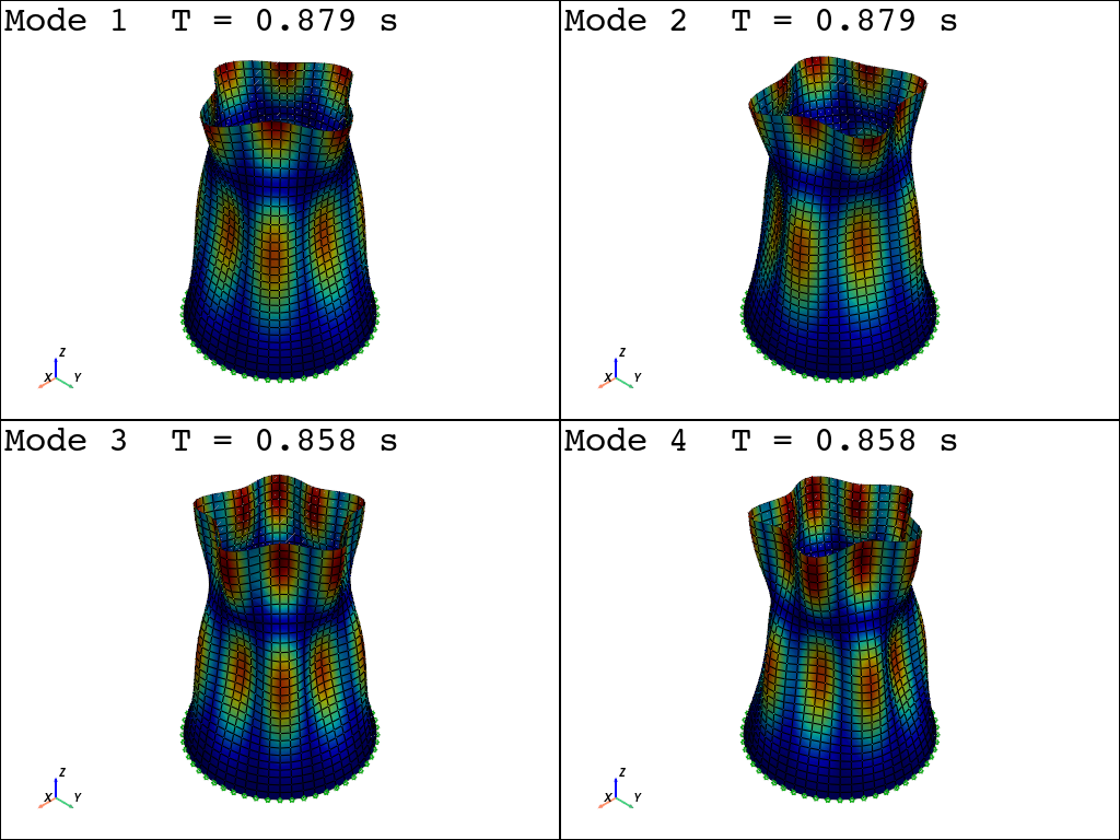
[44]:
fig = opst.vis.pyvista.plot_eigen(mode_tags=4, odb_tag="eigen", subplots=True)
fig.show(jupyter_backend="jupyterlab")
OPSTOOL :: Loading eigen data from _OPSTOOL_ODB/EigenData-eigen.nc ...
[45]:
modal_props, eigen_vectors = opst.post.get_eigen_data(odb_tag="eigen")
modal_props = modal_props.to_pandas()
modal_props.head()
OPSTOOL :: Loading eigen data from _OPSTOOL_ODB/EigenData-eigen.nc ...
[45]:
| Properties | eigenLambda | eigenOmega | eigenFrequency | eigenPeriod | partiFactorMX | partiFactorMY | partiFactorRMZ | partiFactorMZ | partiFactorRMX | partiFactorRMY | ... | partiMassRatiosRMZ | partiMassRatiosMZ | partiMassRatiosRMX | partiMassRatiosRMY | partiMassRatiosCumuMX | partiMassRatiosCumuMY | partiMassRatiosCumuRMZ | partiMassRatiosCumuMZ | partiMassRatiosCumuRMX | partiMassRatiosCumuRMY |
|---|---|---|---|---|---|---|---|---|---|---|---|---|---|---|---|---|---|---|---|---|---|
| modeTags | |||||||||||||||||||||
| 1 | 51.13809 | 7.151090 | 1.138131 | 0.878633 | -1.725009e-11 | 9.416032e-11 | 7.580143e-10 | 4.230678e-12 | 1.235457e-09 | -2.732507e-09 | ... | 1.305012e-27 | 7.354305e-29 | 2.533148e-27 | 1.239162e-26 | 1.222656e-27 | 3.642986e-26 | 1.305012e-27 | 7.354305e-29 | 2.533148e-27 | 1.239162e-26 |
| 2 | 51.13809 | 7.151090 | 1.138131 | 0.878633 | 3.297836e-10 | -3.389637e-10 | 7.606061e-10 | -1.893008e-11 | 1.393822e-08 | 1.180687e-08 | ... | 1.313952e-27 | 1.472403e-27 | 3.224185e-25 | 2.313529e-25 | 4.480913e-25 | 5.085234e-25 | 2.618964e-27 | 1.545946e-27 | 3.249516e-25 | 2.437445e-25 |
| 3 | 53.64215 | 7.324080 | 1.165664 | 0.857880 | -3.402908e-10 | -9.157581e-12 | 1.763309e-09 | -1.133069e-12 | -1.986839e-10 | -1.388419e-08 | ... | 7.061824e-27 | 5.275148e-30 | 6.551348e-29 | 3.199237e-25 | 9.238887e-25 | 5.088680e-25 | 9.680788e-27 | 1.551221e-27 | 3.250171e-25 | 5.636682e-25 |
| 4 | 53.64215 | 7.324080 | 1.165664 | 0.857880 | 4.031667e-10 | -1.081433e-10 | 2.721245e-09 | -1.193286e-11 | 3.973242e-09 | 1.569658e-08 | ... | 1.681880e-26 | 5.850744e-28 | 2.619965e-26 | 4.088982e-25 | 1.591757e-24 | 5.569210e-25 | 2.649959e-26 | 2.136296e-27 | 3.512168e-25 | 9.725664e-25 |
| 5 | 59.58843 | 7.719354 | 1.228573 | 0.813952 | -5.355825e-10 | 2.271784e-10 | -6.861083e-10 | 5.201697e-12 | -1.023211e-08 | -2.045787e-08 | ... | 1.069166e-27 | 1.111762e-28 | 1.737544e-25 | 6.945862e-25 | 2.770379e-24 | 7.689795e-25 | 2.756876e-26 | 2.247472e-27 | 5.249711e-25 | 1.667153e-24 |
5 rows × 34 columns
[46]:
modal_props.loc[[1, 47, 48, 60], "eigenFrequency"]
[46]:
modeTags
1     1.138131
47    2.875771
48    2.875771
60    3.196797
Name: eigenFrequency, dtype: float64
You can compare this with Code-Aster, which uses DKT shell elements. See ~ Model C: Modal analysis of a cooling tower