Fiber Section Visualization

class GetFEMdata and FiberSecVis are needed.

import numpy as np
import openseespy.opensees as ops
from opstool import load_ops_examples
from opstool.vis import GetFEMdata, FiberSecVis

Here we load a single-degree-of-freedom example. This SDOF model consists of a fixed node and a free node connected by a zero-length link element using a circular fiber cross-section.

load_ops_examples("SDOF")

Visualization of fiber section geometry information

Get the fiber section data, note that for parameter ele_sec you should enter a list where each item is a element-section pair, e.g. [(1,1),(1,2), (2,1), ….] , i.e. element 1 and 1# integral point section, element 1 and 2# integral point section, etc.

Method get_fiber_data() will save all fiber data in ele_sec.

Since this is a single-degree-of-freedom model, we have only one link element and one cross section, so enter [(1,1)].

FEMdata = GetFEMdata()

FEMdata.get_fiber_data(ele_sec=[(1, 1)], save_file='FiberData.hdf5')

Fiber section data saved in opstool_output/FiberData.hdf5!

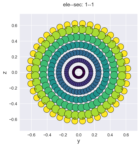
Visualization of fiber cross-sections by sec_vis(). Since only the location and area information of the fiber points can be extracted, a series of circles is used for rendering.

secvis = FiberSecVis(ele_tag=1, sec_tag=1, opacity=1, colormap='viridis')

secvis.sec_vis(input_file='FiberData.hdf5')

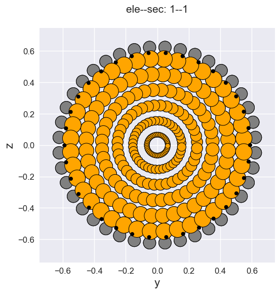
Of course, you can also use a custom color dict, where the keys are the OpenSeesPy material tags in the cross section and the values are any matplotlib supported color labels.

secvis.sec_vis(input_file='FiberData.hdf5',
               mat_color={1: 'gray', 2: 'orange', 3: 'black'})

Fiber section responses visualization

applying the dynamic load

# --------------------------------------------------
# dynamic load
ops.rayleigh(0.0, 0.0, 0.0, 0.000625)
ops.loadConst('-time', 0.0)

# applying Dynamic Ground motion analysis
dt = 0.02
ttot = 5
npts = int(ttot / dt)
x = np.linspace(0, ttot, npts)
data = np.sin(2 * np.pi * x)
ops.timeSeries('Path', 2, '-dt', dt, '-values', *data, '-factor', 9.81)
# how to give accelseriesTag?
ops.pattern('UniformExcitation', 2, 1, '-accel', 2)
# how to give accelseriesTag?
ops.pattern('UniformExcitation', 3, 2, '-accel', 2)

ops.wipeAnalysis()
ops.system('BandGeneral')
# Create the constraint handler, the transformation method
ops.constraints('Transformation')
# Create the DOF numberer, the reverse Cuthill-McKee algorithm
ops.numberer('RCM')
ops.test('NormDispIncr', 1e-8, 10)
ops.algorithm('Linear')
ops.integrator('Newmark', 0.5, 0.25)
ops.analysis('Transient')

Get the response data for each analysis step.

Note

get_fiber_resp_step() can be used with get_node_resp_step() and get_frame_resp_step() at the same time. And the analysis step data reading command that may be added in future versions.

for i in range(npts):
    ops.analyze(1, dt)
    FEMdata.get_fiber_resp_step(num_steps=npts,
                                total_time=100000000000,
                                stop_cond=False,
                                save_file="FiberRespStepData-1.hdf5")

Fiber section responses data saved in opstool_output/FiberRespStepData-1.hdf5!

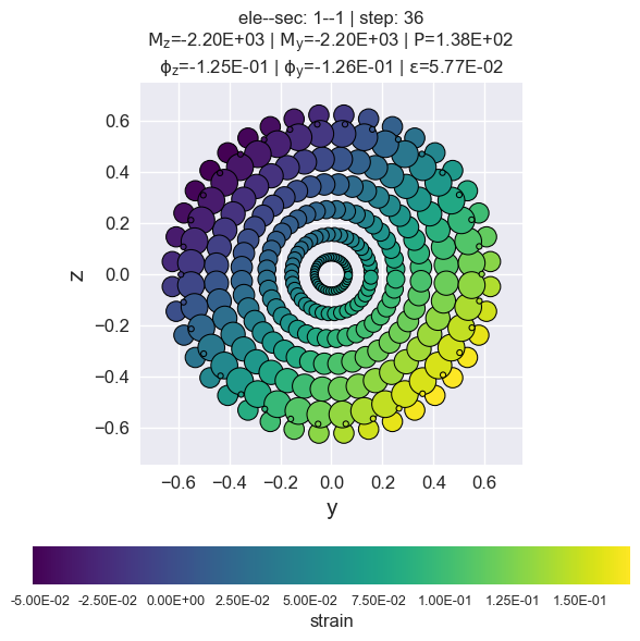
Visualization of the maximum response step if step is None.

resp_vis() can accept the show_variable as “stress” or “strain”. show_mats can be set if you only want to display the response of some materials, the elements must be the material tags that have been defined in the previous opensees commands, and must be included in this section.

secvis.resp_vis(input_file="FiberRespStepData-1.hdf5",
                step=None,
                show_variable='strain',
                show_mats=[1, 2, 3],)

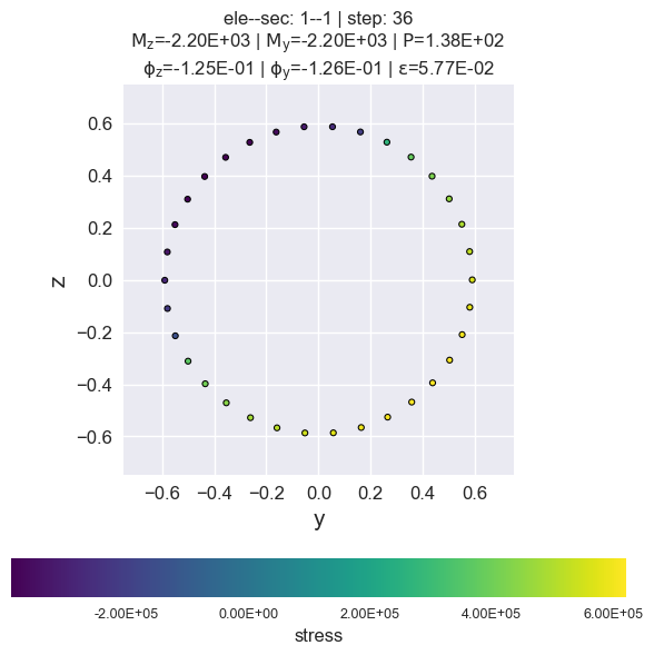
stress of rebars by matTag 3

secvis.resp_vis(input_file="FiberRespStepData-1.hdf5",
                step=None,
                show_variable='stress',
                show_mats=[3],)

Generate animated gif files.

secvis.animation(input_file="FiberRespStepData-1.hdf5",
                 output_file='images/sec1-1.gif',
                 show_variable='strain',
                 show_mats=[1, 2, 3],
                 framerate=10)